In Class Exercise 2: Geospatial Data Wrangling

Published

January 16, 2023

Modified

April 19, 2023

1 Scenario:

Water is an important resource to mankind. Clean and accessible water is critical to human health. It provides a healthy environment, a sustainable economy, reduces poverty and ensures peace and security. Yet over 40% of the global population does not have access to sufficient clean water. By 2025, 1.8 billion people will be living in countries or regions with absolute water scarcity, according to UN-Water. The lack of water poses a major threat to several sectors, including food security. Agriculture uses about 70% of the world’s accessible freshwater.

Developing countries are most affected by water shortages and poor water quality. Up to 80% of illnesses in the developing world are linked to inadequate water and sanitation. Despite technological advancement, providing clean water to the rural community is still a major development issues in many countries globally, especially countries in the Africa continent.

To address the issue of providing clean and sustainable water supply to the rural community, a global Water Point Data Exchange (WPdx) project has been initiated. The main aim of this initiative is to collect water point related data from rural areas at the water point or small water scheme level and share the data via WPdx Data Repository, a cloud-based data library. What is so special of this project is that data are collected based on WPDx Data Standard.

1.1 The Task:

The specific tasks of this take-home exercise are as follows:

Using appropriate sf method, import the shapefile into R and save it in a simple feature data frame format. Note that there are three Projected Coordinate Systems of Nigeria, they are: EPSG: 26391, 26392, and 26303. You can use any one of them.
Using appropriate tidyr and dplyr methods, derive the proportion of functional and non-functional water point at LGA level.
Combining the geospatial and aspatial data frame into simple feature data frame.
Visualising the distribution of water point by using appropriate analytical visualisation methods.

2 Getting Started: Load packages

pacman::p_load(sf, tidyverse, funModeling)

3 Handling Geospatial Data

##Importing Geospatial

geoBoundaries Data set

Show code

geo_nga <- st_read(dsn = "data/geospatial", layer = "geoBoundaries-NGA-ADM2") |>
  st_transform(crs = 26392)

Reading layer `geoBoundaries-NGA-ADM2' from data source 
  `/Users/junhaoteo/Documents/junhao2309/IS415/In-class_Ex/In-class_Ex02/data/geospatial' 
  using driver `ESRI Shapefile'
Simple feature collection with 774 features and 5 fields
Geometry type: MULTIPOLYGON
Dimension:     XY
Bounding box:  xmin: 2.668534 ymin: 4.273007 xmax: 14.67882 ymax: 13.89442
Geodetic CRS:  WGS 84

NGA Data Set

NGA <- st_read("data/geospatial/",
               layer = "nga_admbnda_adm2_osgof_20190417") %>%
  st_transform(crs = 26392)

Reading layer `nga_admbnda_adm2_osgof_20190417' from data source 
  `/Users/junhaoteo/Documents/junhao2309/IS415/In-class_Ex/In-class_Ex02/data/geospatial' 
  using driver `ESRI Shapefile'
Simple feature collection with 774 features and 16 fields
Geometry type: MULTIPOLYGON
Dimension:     XY
Bounding box:  xmin: 2.668534 ymin: 4.273007 xmax: 14.67882 ymax: 13.89442
Geodetic CRS:  WGS 84

3.1 Importing Aspatial data

Use filter to extract only “Nigeria”

Show code

wp_nga <- read_csv(file = "data/aspatial/WPdx.csv") |>
  filter(`#clean_country_name` == "Nigeria")

4 Converting Aspatial Data into Geospatial

Changes only the “New Georeferenced Column” but maintains wp_nga as a tibble dataframe Method in Hands-On_Ex1 also works

Show code

wp_nga$Geometry = st_as_sfc(wp_nga$`New Georeferenced Column`)

wp_nga

# A tibble: 97,478 × 75
   row_id `#source`      #lat_…¹ #lon_…² #repo…³ #stat…⁴ #wate…⁵ #wate…⁶ #wate…⁷
    <dbl> <chr>            <dbl>   <dbl> <chr>   <chr>   <chr>   <chr>   <chr>  
 1 158721 Federal Minis…    5.07    6.62 02/19/… Yes     Boreho… Well    Mechan…
 2 158892 Federal Minis…    5.09    7.09 02/06/… Yes     Boreho… Well    Hand P…
 3 323117 Federal Minis…    5.91    8.77 08/31/… Yes     Boreho… Well    Hand P…
 4 300176 Federal Minis…    5.23    7.32 05/17/… Yes     Boreho… Well    Mechan…
 5 324346 Federal Minis…    6.88    3.36 08/17/… Yes     Boreho… Well    Mechan…
 6 297273 Federal Minis…    6.59    3.29 05/26/… Yes     Boreho… Well    Mechan…
 7 296853 Federal Minis…    6.60    3.26 06/02/… Yes     Boreho… Well    Mechan…
 8 323866 Federal Minis…    6.20    6.73 09/18/… Yes     Boreho… Well    Mechan…
 9 297044 Federal Minis…    6.61    3.30 05/26/… Yes     Boreho… Well    Mechan…
10 324321 Federal Minis…    6.96    3.60 08/16/… Yes     Boreho… Well    Mechan…
# … with 97,468 more rows, 66 more variables: `#water_tech_category` <chr>,
#   `#facility_type` <chr>, `#clean_country_name` <chr>, `#clean_adm1` <chr>,
#   `#clean_adm2` <chr>, `#clean_adm3` <chr>, `#clean_adm4` <chr>,
#   `#install_year` <dbl>, `#installer` <chr>, `#rehab_year` <lgl>,
#   `#rehabilitator` <chr>, `#management_clean` <chr>, `#status_clean` <chr>,
#   `#pay` <chr>, `#fecal_coliform_presence` <chr>,
#   `#fecal_coliform_value` <dbl>, `#subjective_quality` <chr>, …

Convert wp_NGA into an sf data.frame and transforming it into the Nigeria projected coordinate system

Show code

wp_sf <- st_sf(wp_nga, crs = 4326) |>
  st_transform(crs = 26392)
wp_sf

Simple feature collection with 97478 features and 74 fields
Geometry type: POINT
Dimension:     XY
Bounding box:  xmin: 28907.91 ymin: 33736.93 xmax: 1293293 ymax: 1092883
Projected CRS: Minna / Nigeria Mid Belt
# A tibble: 97,478 × 75
   row_id `#source`      #lat_…¹ #lon_…² #repo…³ #stat…⁴ #wate…⁵ #wate…⁶ #wate…⁷
 *  <dbl> <chr>            <dbl>   <dbl> <chr>   <chr>   <chr>   <chr>   <chr>  
 1 158721 Federal Minis…    5.07    6.62 02/19/… Yes     Boreho… Well    Mechan…
 2 158892 Federal Minis…    5.09    7.09 02/06/… Yes     Boreho… Well    Hand P…
 3 323117 Federal Minis…    5.91    8.77 08/31/… Yes     Boreho… Well    Hand P…
 4 300176 Federal Minis…    5.23    7.32 05/17/… Yes     Boreho… Well    Mechan…
 5 324346 Federal Minis…    6.88    3.36 08/17/… Yes     Boreho… Well    Mechan…
 6 297273 Federal Minis…    6.59    3.29 05/26/… Yes     Boreho… Well    Mechan…
 7 296853 Federal Minis…    6.60    3.26 06/02/… Yes     Boreho… Well    Mechan…
 8 323866 Federal Minis…    6.20    6.73 09/18/… Yes     Boreho… Well    Mechan…
 9 297044 Federal Minis…    6.61    3.30 05/26/… Yes     Boreho… Well    Mechan…
10 324321 Federal Minis…    6.96    3.60 08/16/… Yes     Boreho… Well    Mechan…
# … with 97,468 more rows, 66 more variables: `#water_tech_category` <chr>,
#   `#facility_type` <chr>, `#clean_country_name` <chr>, `#clean_adm1` <chr>,
#   `#clean_adm2` <chr>, `#clean_adm3` <chr>, `#clean_adm4` <chr>,
#   `#install_year` <dbl>, `#installer` <chr>, `#rehab_year` <lgl>,
#   `#rehabilitator` <chr>, `#management_clean` <chr>, `#status_clean` <chr>,
#   `#pay` <chr>, `#fecal_coliform_presence` <chr>,
#   `#fecal_coliform_value` <dbl>, `#subjective_quality` <chr>, …

5 Geospatial Data Cleaning

##Exclude redundent fields

Show code

NGA <- NGA %>%
  select(c(3:4, 8:9))

5.1 Checking duplicate name and amending them

NGA$ADM2_EN[duplicated(NGA$ADM2_EN) == TRUE]

[1] "Bassa"    "Ifelodun" "Irepodun" "Nasarawa" "Obi"      "Surulere"

Correct the areas as they are located in different states

NGA$ADM2_EN[94] <- "Bassa, Kogi"
NGA$ADM2_EN[95] <- "Bassa, Plateau"
NGA$ADM2_EN[304] <- "Ifelodun, Kwara"
NGA$ADM2_EN[305] <- "Ifelodun, Osun"
NGA$ADM2_EN[355] <- "Irepodun, Kwara"
NGA$ADM2_EN[356] <- "Irepodun, Osun"
NGA$ADM2_EN[519] <- "Nasarawa, Kano"
NGA$ADM2_EN[520] <- "Nasarawa, Nasarawa"
NGA$ADM2_EN[546] <- "Obi, Benue"
NGA$ADM2_EN[547] <- "Obi, Nasarawa"
NGA$ADM2_EN[693] <- "Surulere, Lagos"
NGA$ADM2_EN[694] <- "Surulere, Oyo"

Rerun code to check

Show code

NGA$ADM2_EN[duplicated(NGA$ADM2_EN) == TRUE]

character(0)

6 Data Wrangling for Water Point Data

freq() showcase the distribution of waterpoint status visually.

freq(data = wp_sf,
     input = '#status_clean')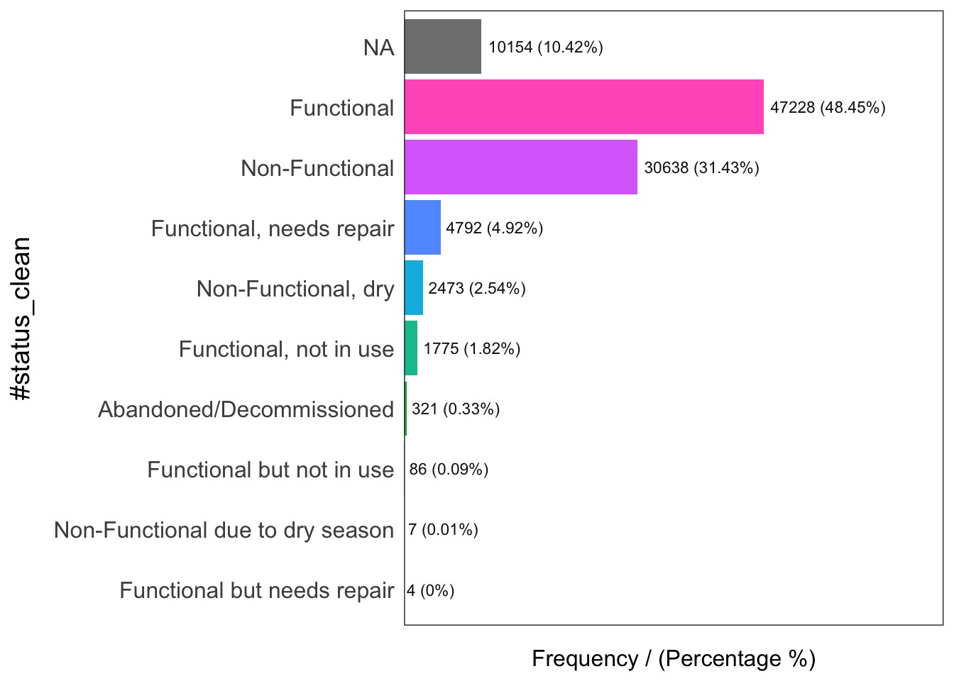

                      #status_clean frequency percentage cumulative_perc
1                        Functional     47228      48.45           48.45
2                    Non-Functional     30638      31.43           79.88
3                              <NA>     10154      10.42           90.30
4          Functional, needs repair      4792       4.92           95.22
5               Non-Functional, dry      2473       2.54           97.76
6            Functional, not in use      1775       1.82           99.58
7          Abandoned/Decommissioned       321       0.33           99.91
8         Functional but not in use        86       0.09          100.00
9  Non-Functional due to dry season         7       0.01          100.01
10      Functional but needs repair         4       0.00          100.00

replace_na(status_clean, “unknown”) : replaces all NA to unknown within status_clean variable

wp_sf_nga <- wp_sf %>%
  rename(status_clean = '#status_clean') %>%
  select(status_clean) %>%
  mutate(status_clean = replace_na(
    status_clean, 'unknown'))

6.1 Extracting Water Point Data

Filter based on functional, non_functional and unknown respectively.

wp_functional <- wp_sf_nga %>%
  filter(status_clean %in%
           c("Functional",
             "Functional but not in use",
             "Functional but needs repair"))

wp_nonfunctional <- wp_sf_nga %>% 
  filter(status_clean %in% 
           c("Abandoned/Decommissioned",
             "Abandoned",
             "Non-Functional due to dry season",
             "Non-Functional",
             "Non functional due to dry season"))

wp_unknown <- wp_sf_nga %>%
  filter(status_clean %in% "unknown")

freq(data = wp_functional,
     input = 'status_clean')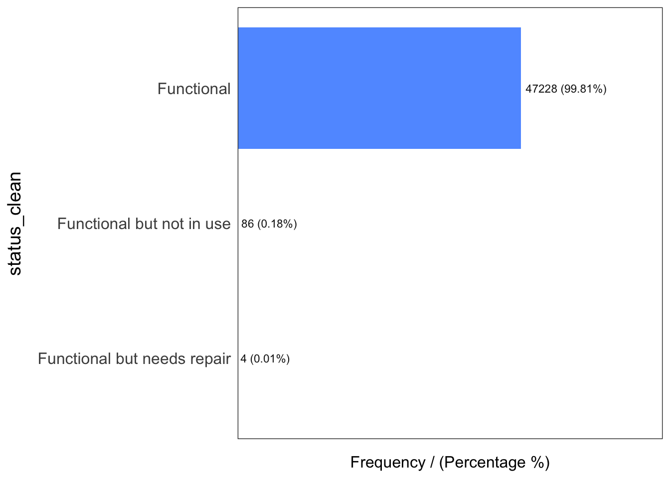

                 status_clean frequency percentage cumulative_perc
1                  Functional     47228      99.81           99.81
2   Functional but not in use        86       0.18           99.99
3 Functional but needs repair         4       0.01          100.00

freq(data = wp_nonfunctional,
     input = 'status_clean')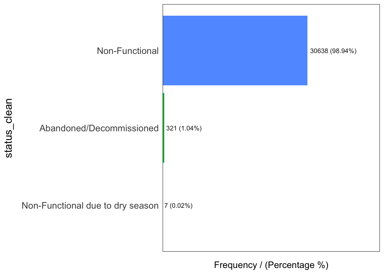

                      status_clean frequency percentage cumulative_perc
1                   Non-Functional     30638      98.94           98.94
2         Abandoned/Decommissioned       321       1.04           99.98
3 Non-Functional due to dry season         7       0.02          100.00

freq(data = wp_unknown,
     input = 'status_clean')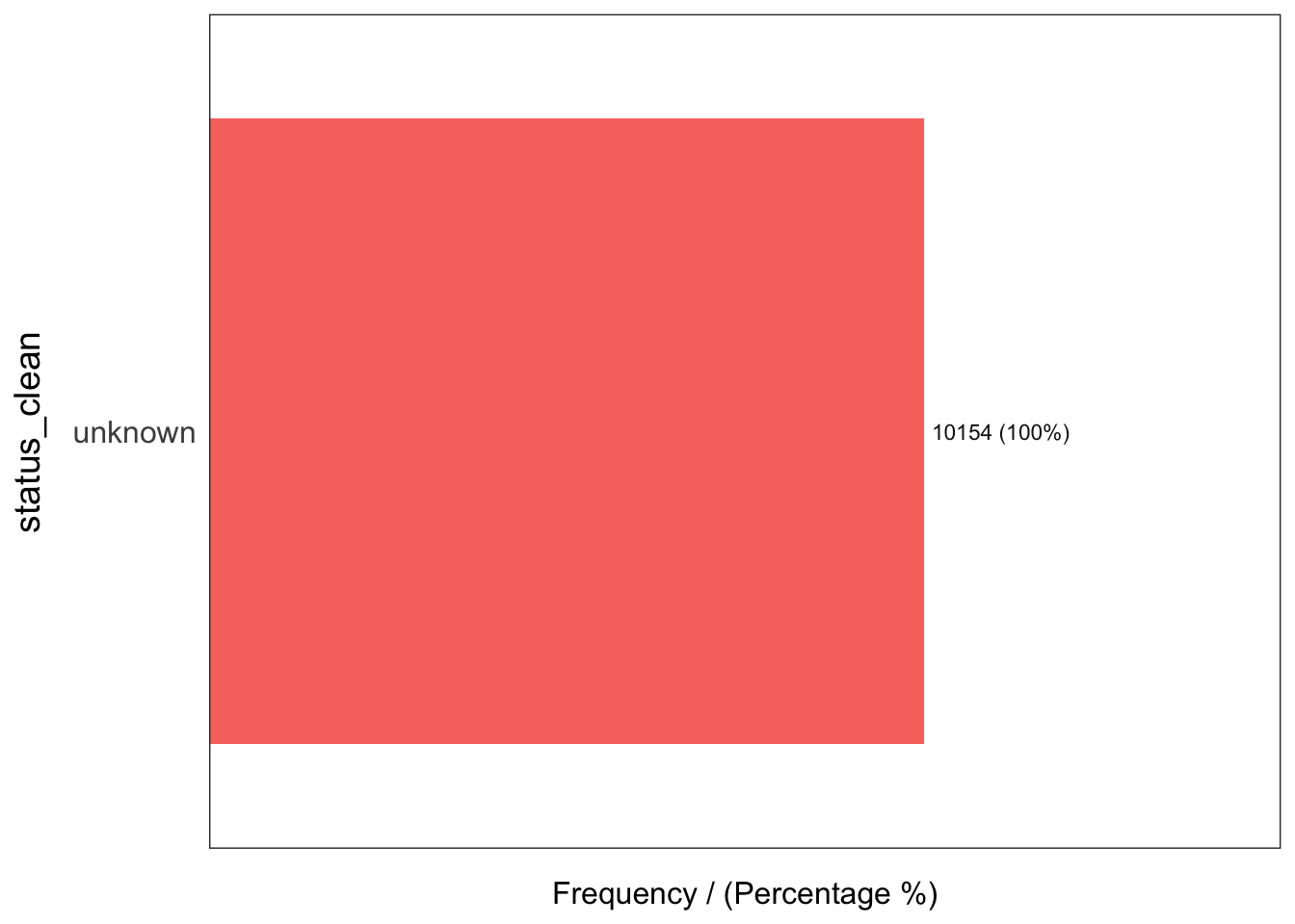

  status_clean frequency percentage cumulative_perc
1      unknown     10154        100             100

6.2 Performing Point-in-Polygon Count

NGA_wp <- NGA %>%
  mutate(`total_wp` = lengths(
    st_intersects(NGA, wp_sf_nga))) %>%
  mutate(`wp_functional` = lengths(
    st_intersects(NGA, wp_functional))) %>%
  mutate(`wp_nonfunctional` = lengths(
    st_intersects(NGA, wp_nonfunctional))) %>%
  mutate(`wp_unknown` = lengths(
    st_intersects(NGA, wp_unknown)))

6.3 Visualing attributes by using statistical graph

Show code

ggplot(data = NGA_wp,
       aes(x = total_wp)) +
  geom_histogram(bins = 20, 
                 color = "black",
                 fill ="light blue") +
  geom_vline(aes(xintercept=mean(total_wp, na.rm=T)),
             color = "red", linetype="dashed", size = 0.8) +
  xlab("No of water points") +
  ylab("No. of\nLGAs") +
  theme(axis.title.y = element_text(angle = 0))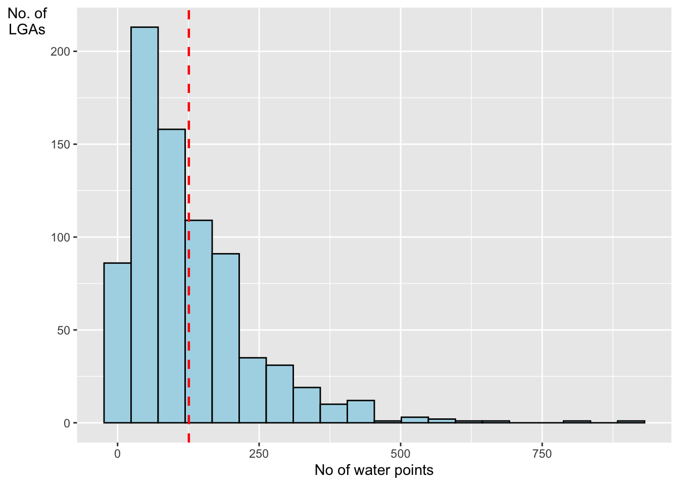

Show code

write_rds(NGA_wp, "data/rds/NGA_wp.rds")