pacman::p_load(tidyverse, sf, sfdep, tmap, httr, jsonlite, matrixStats, readr, GWmodel, SpatialML, rsample, Metrics)Take-home Exercise 3: Predicting HDB Public Housing Resale Pricies using Geographically Weighted Methods
1 Setting the Scene
Housing is an essential component of household wealth worldwide. Buying a housing has always been a major investment for most people. The price of housing is affected by many factors. Some of them are global in nature such as the general economy of a country or inflation rate. Others can be more specific to the properties themselves. These factors can be further divided to structural and locational factors. Structural factors are variables related to the property themselves such as the size, fitting, and tenure of the property. Locational factors are variables related to the neighbourhood of the properties such as proximity to childcare centre, public transport service and shopping centre.
Conventional, housing resale prices predictive models were built by using Ordinary Least Square (OLS) method. However, this method failed to take into consideration that spatial autocorrelation and spatial heterogeneity exist in geographic data sets such as housing transactions. With the existence of spatial autocorrelation, the OLS estimation of predictive housing resale pricing models could lead to biased, inconsistent, or inefficient results (Anselin 1998). In view of this limitation, Geographical Weighted Models were introduced for calibrating predictive model for housing resale prices.
1.1 The Task
In this take-home exercise, I am tasked to predict HDB resale prices at the sub-market level (HDB 5-room) for the month of January and February 2023 in Singapore. The predictive models must be built by using by using conventional OLS method and GWR methods. The data set used to train the model is from January 2021 to December 2022.
1.2 Packages used:
The R packages we’ll use for this analysis are:
sf: used for importing, managing, and processing geospatial data
tidyverse: a collection of packages for data science tasks
tmap: used for creating thematic maps, such as choropleth and bubble maps
spdep: used to create spatial weights matrix objects, global and local spatial autocorrelation statistics and related calculations (e.g. spatially lag attributes)
onemapsgapi: used to query Singapore-specific spatial data, alongside additional functionalities. Recommended readings: Vignette and Documentation
httr : used to make API calls, such as a GET request
units: used to for manipulating numeric vectors that have physical measurement units associated with them
matrixStats: a set of high-performing functions for operating on rows and columns of matrices
jsonlite: a JSON parser that can convert from JSON to the appropriate R data types
corrplot + ggpubr: both are used for multivariate data visualisation & analysis
GWmodel: provides a collection of localised spatial statistical methods, such as summary statistics, principal components analysis, discriminant analysis and various forms of GW regression
kableExtra: an extension of kable, used for table customisation
The following tidyverse packages will be used:
readr for importing delimited files (.csv)
tidyr for manipulating and tidying data
dplyr for wrangling and transforming data
ggplot2 for visualising data
1.3 Data used:
Show code
# initialise a dataframe of our aspatial and geospatial dataset details
datasets <- data.frame(
  Type=c("Aspatial",
         "Geospatial",
         "Geospatial",
         "Geospatial",

         "Geospatial - Onemap",
         "Geospatial - Onemap",
         "Geospatial - Onemap",
         "Geospatial - Onemap",
         "Geospatial - Onemap",
         "Geospatial - Onemap",
         "Geospatial - Onemap",
         "Geospatial - Onemap",
         "Geospatial - Onemap",

         "Aspatial - Self-Sourced",
         "Aspatial - Self-Sourced"),

  Name=c("Resale Flat Prices",
         "Master Plan 2019 Subzone Boundary (Web)",
         "MRT & LRT Exit Locations",
         "Bus Stop Locations",

         "Childcare Services",
         "Eldercare Services",
         "Hawker Centres",
         "Kindergartens",
         "Parks",
         "Supermarkets",
         "Community Clubs",
         "Family Services",
         "Registered Pharmacies",

         "Schools",
         "Shopping Mall SVY21 Coordinates`"),

  Format=c(".csv",
           ".shp",
           ".shp",
           ".shp",

           ".shp",
           ".shp",
           ".shp",
           ".shp",
           ".shp",
           ".shp",
           ".shp",
           ".shp",
           ".shp",

           ".csv",
           ".csv"),

  Source=c("[data.gov.sg](https://data.gov.sg/dataset/resale-flat-prices)",
           "data.gov.sg",
           "[LTA Data Mall](https://datamall.lta.gov.sg/content/datamall/en/search_datasets.html?searchText=Train)",
           "[LTA Data Mall](https://datamall.lta.gov.sg/content/datamall/en/search_datasets.html?searchText=bus%20stop)",

           "[OneMap API]",
           "[OneMap API](https://www.onemap.gov.sg/docs/)",
           "[OneMap API](https://www.onemap.gov.sg/docs/)",
           "[OneMap API](https://www.onemap.gov.sg/docs/)",
           "[OneMap API](https://www.onemap.gov.sg/docs/)",
           "[OneMap API](https://www.onemap.gov.sg/docs/)",
           "[OneMap API](https://www.onemap.gov.sg/docs/)",
           "[OneMap API](https://www.onemap.gov.sg/docs/)",
           "[OneMap API](https://www.onemap.gov.sg/docs/)",

           "[data.gov.sg](https://data.gov.sg/dataset/school-directory-and-information)",
           "[Mall SVY21 Coordinates Web Scaper](https://github.com/ValaryLim/Mall-Coordinates-Web-Scraper)")
  )

# with reference to this guide on kableExtra:
# https://cran.r-project.org/web/packages/kableExtra/vignettes/awesome_table_in_html.html
# kable_material is the name of the kable theme
# 'hover' for to highlight row when hovering, 'scale_down' to adjust table to fit page width
library(knitr)
library(kableExtra)
kable(datasets, caption="Datasets Used") %>%
kable_material("hover", latex_options="scale_down")| Type | Name | Format | Source |
|---|---|---|---|
| Aspatial | Resale Flat Prices | .csv | [data.gov.sg](https://data.gov.sg/dataset/resale-flat-prices) |
| Geospatial | Master Plan 2019 Subzone Boundary (Web) | .shp | data.gov.sg |
| Geospatial | MRT & LRT Exit Locations | .shp | [LTA Data Mall](https://datamall.lta.gov.sg/content/datamall/en/search_datasets.html?searchText=Train) |
| Geospatial | Bus Stop Locations | .shp | [LTA Data Mall](https://datamall.lta.gov.sg/content/datamall/en/search_datasets.html?searchText=bus%20stop) |
| Geospatial - Onemap | Childcare Services | .shp | [OneMap API] |
| Geospatial - Onemap | Eldercare Services | .shp | [OneMap API](https://www.onemap.gov.sg/docs/) |
| Geospatial - Onemap | Hawker Centres | .shp | [OneMap API](https://www.onemap.gov.sg/docs/) |
| Geospatial - Onemap | Kindergartens | .shp | [OneMap API](https://www.onemap.gov.sg/docs/) |
| Geospatial - Onemap | Parks | .shp | [OneMap API](https://www.onemap.gov.sg/docs/) |
| Geospatial - Onemap | Supermarkets | .shp | [OneMap API](https://www.onemap.gov.sg/docs/) |
| Geospatial - Onemap | Community Clubs | .shp | [OneMap API](https://www.onemap.gov.sg/docs/) |
| Geospatial - Onemap | Family Services | .shp | [OneMap API](https://www.onemap.gov.sg/docs/) |
| Geospatial - Onemap | Registered Pharmacies | .shp | [OneMap API](https://www.onemap.gov.sg/docs/) |
| Aspatial - Self-Sourced | Schools | .csv | [data.gov.sg](https://data.gov.sg/dataset/school-directory-and-information) |
| Aspatial - Self-Sourced | Shopping Mall SVY21 Coordinates` | .csv | [Mall SVY21 Coordinates Web Scaper](https://github.com/ValaryLim/Mall-Coordinates-Web-Scraper) |
1.3.1 How to extract data from onemap
These are the steps:
The code chunks below uses onemapsgapi package.
- Register an account with onemap
- A code is then be sent to your email. Then fill in this form
- In the console, run the code chunk below:
token <- get_token("email", "password")Input the email and password that you’ve registered with onemap. This will provide you a token ID under objectname: token. Note that you will need to do this again as the token is only valid for 3 days.
- Obtain queryname by running the code chunk below:
themes <- search_themes(token)Input your token ID and you can source for the queryname for Step 5.
- Use get_theme() to get the data from onemap
For this example, we will use queryname, “eldercare”.
eldercare<-get_theme(token,"eldercare")- Convert the object into an sf object then download it into your data folder. st_as_sf() is for converting the file and st_write() is for writing the file into your folder. st_transform() sets the coordinate reference system to Singapore, EPSG::3414. These functions are from the sf package.
eldercaresf <- st_as_sf(eldercare, coords=c("Lng", "Lat"),
                        crs=4326) %>%
  st_transform(crs = 3414)
st_write(obj = eldercaresf,
         dsn = "data/geospatial",
         layer = "eldercare",
         driver = "ESRI Shapefile")
To make it more automatic, define which variables you want from the onemap database into a vector. The code chunk runs a for loop that does steps 5 and 6 together and stores them into your folder.
onemap_variables <- c("childcare", "communityclubs", "eldercare", "family", "hawkercentre", "kindergartens", "nationalparks","registered_pharmacy","supermarkets")

df <- list()
df_sf <- list()
for (i in 1:length(onemap_variables)){
  df[[i]] <- get_theme(token, onemap_variables[i])
  df_sf[[i]] <- st_as_sf(df[[i]], coords=c("Lng", "Lat"),
                        crs=4326) %>%
    st_transform(crs = 3414)
st_write(obj = df_sf[[i]],
         dsn = "data/geospatial/Onemap",
         layer = onemap_variables[i],
         driver = "ESRI Shapefile")
}
2 Load Data into R
2.1 Geospatial Data
We will make use of st_read() from the sf package to load the data in
pharmacy <- st_read(dsn = "data/geospatial/Onemap",
                layer = "registered_pharmacy")
Reading layer `registered_pharmacy' from data source
`/Users/junhaoteo/Documents/junhao2309/IS415/Take-Home_Ex/Take-Home_Ex03/data/geospatial/Onemap'
using driver `ESRI Shapefile'
Simple feature collection with 269 features and 8 fields
Geometry type: POINT
Dimension: XY
Bounding box: xmin: 13049.46 ymin: 26540.77 xmax: 46829.34 ymax: 47763.05
Projected CRS: SVY21 / Singapore TMparks <- st_read(dsn = "data/geospatial/Onemap",
layer = "nationalparks")Reading layer `nationalparks' from data source
`/Users/junhaoteo/Documents/junhao2309/IS415/Take-Home_Ex/Take-Home_Ex03/data/geospatial/Onemap'
using driver `ESRI Shapefile'
Simple feature collection with 421 features and 2 fields
Geometry type: POINT
Dimension: XY
Bounding box: xmin: 12374.75 ymin: 21917.81 xmax: 52533.09 ymax: 49296.46
Projected CRS: SVY21 / Singapore TMkindergartens <- st_read(dsn = "data/geospatial/Onemap",
layer = "kindergartens")Reading layer `kindergartens' from data source
`/Users/junhaoteo/Documents/junhao2309/IS415/Take-Home_Ex/Take-Home_Ex03/data/geospatial/Onemap'
using driver `ESRI Shapefile'
Simple feature collection with 448 features and 5 fields
Geometry type: POINT
Dimension: XY
Bounding box: xmin: 11909.7 ymin: 25596.33 xmax: 43395.47 ymax: 48562.06
Projected CRS: SVY21 / Singapore TMhawker <- st_read(dsn = "data/geospatial/Onemap",
layer = "hawkercentre")Reading layer `hawkercentre' from data source
`/Users/junhaoteo/Documents/junhao2309/IS415/Take-Home_Ex/Take-Home_Ex03/data/geospatial/Onemap'
using driver `ESRI Shapefile'
Simple feature collection with 125 features and 18 fields
Geometry type: POINT
Dimension: XY
Bounding box: xmin: 12874.19 ymin: 28355.97 xmax: 45241.4 ymax: 47850.43
Projected CRS: SVY21 / Singapore TMeldercare <- st_read(dsn = "data/geospatial/Onemap",
layer = "eldercare")Reading layer `eldercare' from data source
`/Users/junhaoteo/Documents/junhao2309/IS415/Take-Home_Ex/Take-Home_Ex03/data/geospatial/Onemap'
using driver `ESRI Shapefile'
Simple feature collection with 133 features and 4 fields
Geometry type: POINT
Dimension: XY
Bounding box: xmin: 14481.92 ymin: 28218.43 xmax: 41665.14 ymax: 46804.9
Projected CRS: SVY21 / Singapore TMcommunityclubs <-st_read(dsn = "data/geospatial/Onemap",
layer = "communityclubs")Reading layer `communityclubs' from data source
`/Users/junhaoteo/Documents/junhao2309/IS415/Take-Home_Ex/Take-Home_Ex03/data/geospatial/Onemap'
using driver `ESRI Shapefile'
Simple feature collection with 125 features and 11 fields
Geometry type: POINT
Dimension: XY
Bounding box: xmin: 12308.4 ymin: 28593.37 xmax: 42008.87 ymax: 48958.52
Projected CRS: SVY21 / Singapore TMsupermarkets <- st_read(dsn = "data/geospatial/Onemap",
layer = "SUPERMARKETS")Reading layer `SUPERMARKETS' from data source
`/Users/junhaoteo/Documents/junhao2309/IS415/Take-Home_Ex/Take-Home_Ex03/data/geospatial/Onemap'
using driver `ESRI Shapefile'
Simple feature collection with 526 features and 8 fields
Geometry type: POINT
Dimension: XY
Bounding box: xmin: 4901.188 ymin: 25529.08 xmax: 46948.22 ymax: 49233.6
Projected CRS: SVY21familyservices <- st_read(dsn = "data/geospatial/Onemap",
layer = "family")Reading layer `family' from data source
`/Users/junhaoteo/Documents/junhao2309/IS415/Take-Home_Ex/Take-Home_Ex03/data/geospatial/Onemap'
using driver `ESRI Shapefile'
Simple feature collection with 48 features and 7 fields
Geometry type: POINT
Dimension: XY
Bounding box: xmin: 12836.2 ymin: 28549.79 xmax: 42512.91 ymax: 47397.09
Projected CRS: SVY21 / Singapore TMchildcare <- st_read(dsn = "data/geospatial/Onemap",
layer = "childcare")Reading layer `childcare' from data source
`/Users/junhaoteo/Documents/junhao2309/IS415/Take-Home_Ex/Take-Home_Ex03/data/geospatial/Onemap'
using driver `ESRI Shapefile'
Simple feature collection with 1925 features and 5 fields
Geometry type: POINT
Dimension: XY
Bounding box: xmin: 11810.03 ymin: 25596.33 xmax: 45404.24 ymax: 49300.88
Projected CRS: SVY21 / Singapore TMWe will make use of st_read() from the sf package to load the data in
mpsz <- st_read(dsn = "data/geospatial",
                layer = "MP14_SUBZONE_WEB_PL")
Reading layer `MP14_SUBZONE_WEB_PL' from data source
`/Users/junhaoteo/Documents/junhao2309/IS415/Take-Home_Ex/Take-Home_Ex03/data/geospatial'
using driver `ESRI Shapefile'
Simple feature collection with 323 features and 15 fields
Geometry type: MULTIPOLYGON
Dimension: XY
Bounding box: xmin: 2667.538 ymin: 15748.72 xmax: 56396.44 ymax: 50256.33
Projected CRS: SVY21We will make use of st_read() from the sf package to load the data in
Bus_stop <- st_read(dsn = "data/geospatial",
                layer = "BusStop")
Reading layer `BusStop' from data source
`/Users/junhaoteo/Documents/junhao2309/IS415/Take-Home_Ex/Take-Home_Ex03/data/geospatial'
using driver `ESRI Shapefile'
Simple feature collection with 5159 features and 3 fields
Geometry type: POINT
Dimension: XY
Bounding box: xmin: 3970.122 ymin: 26482.1 xmax: 48284.56 ymax: 52983.82
Projected CRS: SVY21MRT <- st_read(dsn = "data/geospatial/lta-mrt-station-exit-kml.kml")Reading layer `MRT_EXITS' from data source
`/Users/junhaoteo/Documents/junhao2309/IS415/Take-Home_Ex/Take-Home_Ex03/data/geospatial/lta-mrt-station-exit-kml.kml'
using driver `KML'
Simple feature collection with 474 features and 2 fields
Geometry type: POINT
Dimension: XYZ
Bounding box: xmin: 103.6368 ymin: 1.264972 xmax: 103.9893 ymax: 1.449157
z_range: zmin: 0 zmax: 0
Geodetic CRS: WGS 84We will make use of read_csv() from the readr package to read the csv file into Rstudio
Resale <- read_csv("data/aspatial/resale-flat-prices-based-on-registration-date-from-jan-2017-onwards.csv")Schools <- read_csv("data/aspatial/schools.csv")Malls <- read_csv("data/aspatial/mall_coordinates_updated.csv")3 Data Wrangling
3.1 HDB Resale Price
For the purpose of this take-home exercise, we will only be using five-room flat and training transaction period should be from January 2021 and December 2022.
From the output above, the variables we want are:
- Resale Price
- Month
- Flat Type
- Area of the unit
- Floor level
- Remaining Lease
- Flat Model
3.1.1 Story and Date adjustents
We will see the unique values of story by running the code chunk below.
unique(Resale$storey_range) [1] "10 TO 12" "01 TO 03" "04 TO 06" "07 TO 09" "13 TO 15" "19 TO 21"
[7] "22 TO 24" "16 TO 18" "34 TO 36" "28 TO 30" "37 TO 39" "49 TO 51"
[13] "25 TO 27" "40 TO 42" "31 TO 33" "46 TO 48" "43 TO 45"As we can see, there are 17 factor levels.
When dealing with categorical variables, there are several ways to manipulate the data.
These are some ways to deal with categorical variables:
- Set it as a factor, to which R will recognize them as binary variables automatically.
- Set categorical variable as multiple binary variable columns, assigning values 1 and 0.
- Set categorical variables as ordinal numbers.
In the case of story levels, as they are ascending in nature, we can use No. 3, which is to set them as ordinal variables.
The code chunk below will sequence the story levels, assigning value 1 to “01 TO 03”, 2 to “04 TO 06”, …, 17 to “49 TO 51”.
# Define the story levels and ordinal values
story_levels <- c("01 TO 03", "04 TO 06", "07 TO 09", "10 TO 12", "13 TO 15", "16 TO 18", "19 TO 21", "22 TO 24", "25 TO 27", "28 TO 30", "31 TO 33", "34 TO 36", "37 TO 39", "40 TO 42", "43 TO 45", "46 TO 48", "49 TO 51")
story_ordinal <- seq_along(story_levels)

# Create the ordinal variable based on the story column
Resale$Story_Ordinal <- story_ordinal[match(Resale$storey_range, story_levels)]

# Set the labels for the ordinal variable
levels(Resale$Story_Ordinal) <- story_levels
3.1.2 Date
Next we will set the Date column as date type and also ensure Story_Ordinal is of numeric type.
To check the data set, you can run glimpse() from the dplyr package to see the data types of each variable.
Resale <- Resale %>%
  mutate(month = as.Date(paste0(month, "-01"), format ="%Y-%m-%d"),
         Story_Ordinal = as.numeric(Story_Ordinal))
3.1.3 Flat Model
Next, we will set Flat Model as a binary variable by running the code chunk below.
Resale <- Resale %>%
  tidyr::pivot_wider(names_from = flat_model,
              values_from = flat_model,
              values_fn = list(flat_model = ~1),
              values_fill = 0)
3.1.4 Remaining Lease
We will settle the remaining lease by running the code chunk below: This turns remaining_lease from chr type to numeric in terms of units, years.
# Splits the string by year and month, using str_split from the stringr package
str_list <- str_split(Resale$remaining_lease, " ")

for (i in 1:length(str_list)) {
  if (length(unlist(str_list[i])) > 2) {
      year <- as.numeric(unlist(str_list[i])[1])
      month <- as.numeric(unlist(str_list[i])[3])
      Resale$remaining_lease[i] <- year + round(month/12, 2)
  }
  else {
    year <- as.numeric(unlist(str_list[i])[1])
    Resale$remaining_lease[i] <- year
  }
}

Resale <- Resale %>%
  mutate(remaining_lease =as.numeric(remaining_lease))
We can take a look at the dataframe now by using glimpse() from the dplyr package
glimpse(Resale)Rows: 148,000
Columns: 11
$ month <chr> "2017-01", "2017-01", "2017-01", "2017-01", "2017-…
$ town <chr> "ANG MO KIO", "ANG MO KIO", "ANG MO KIO", "ANG MO …
$ flat_type <chr> "2 ROOM", "3 ROOM", "3 ROOM", "3 ROOM", "3 ROOM", …
$ block <chr> "406", "108", "602", "465", "601", "150", "447", "…
$ street_name <chr> "ANG MO KIO AVE 10", "ANG MO KIO AVE 4", "ANG MO K…
$ storey_range <chr> "10 TO 12", "01 TO 03", "01 TO 03", "04 TO 06", "0…
$ floor_area_sqm <dbl> 44, 67, 67, 68, 67, 68, 68, 67, 68, 67, 68, 67, 67…
$ flat_model <chr> "Improved", "New Generation", "New Generation", "N…
$ lease_commence_date <dbl> 1979, 1978, 1980, 1980, 1980, 1981, 1979, 1976, 19…
$ remaining_lease <chr> "61 years 04 months", "60 years 07 months", "62 ye…
$ resale_price <dbl> 232000, 250000, 262000, 265000, 265000, 275000, 28…We will first filter out the relevant columns we want by running the code chunk below:
select() helps to select the columns we want and filter() helps us to filter to the specific two months. These two functions come from the dplyr package.
Resale_train <- Resale %>%
  filter(month >= "2021-01-01" & month <= "2022-12-01",
         flat_type == "5 ROOM") %>%
  dplyr::select(-2,-3,-6,-8)
We will save Resale_train as a rds file for easy retrieval
write_rds(Resale_train, "data/aspatial/Resale_train.rds")Resale_train <- read_rds("data/aspatial/Resale_train.rds")glimpse(Resale_train)Rows: 14,508
Columns: 28
$ month <date> 2021-01-01, 2021-01-01, 2021-01-01, 2021-01-…
$ block <chr> "551", "305", "520", "253", "423", "617", "31…
$ street_name <chr> "ANG MO KIO AVE 10", "ANG MO KIO AVE 1", "ANG…
$ floor_area_sqm <dbl> 118, 123, 118, 128, 133, 133, 110, 110, 110, …
$ remaining_lease <dbl> 59.08, 55.58, 58.67, 74.25, 71.25, 74.50, 84.…
$ resale_price <dbl> 483000, 590000, 629000, 670000, 680000, 76000…
$ Story_Ordinal <dbl> 1, 5, 6, 3, 1, 5, 8, 5, 6, 6, 5, 5, 8, 1, 2, …
$ Improved <dbl> 1, 0, 1, 1, 1, 0, 1, 1, 1, 0, 0, 0, 0, 0, 1, …
$ `New Generation` <dbl> 0, 0, 0, 0, 0, 0, 0, 0, 0, 0, 0, 0, 0, 0, 0, …
$ DBSS <dbl> 0, 0, 0, 0, 0, 0, 0, 0, 0, 1, 1, 1, 1, 0, 0, …
$ Standard <dbl> 0, 1, 0, 0, 0, 0, 0, 0, 0, 0, 0, 0, 0, 1, 0, …
$ Apartment <dbl> 0, 0, 0, 0, 0, 0, 0, 0, 0, 0, 0, 0, 0, 0, 0, …
$ Simplified <dbl> 0, 0, 0, 0, 0, 0, 0, 0, 0, 0, 0, 0, 0, 0, 0, …
$ `Model A` <dbl> 0, 0, 0, 0, 0, 1, 0, 0, 0, 0, 0, 0, 0, 0, 0, …
$ `Premium Apartment` <dbl> 0, 0, 0, 0, 0, 0, 0, 0, 0, 0, 0, 0, 0, 0, 0, …
$ `Adjoined flat` <dbl> 0, 0, 0, 0, 0, 0, 0, 0, 0, 0, 0, 0, 0, 0, 0, …
$ `Model A-Maisonette` <dbl> 0, 0, 0, 0, 0, 0, 0, 0, 0, 0, 0, 0, 0, 0, 0, …
$ Maisonette <dbl> 0, 0, 0, 0, 0, 0, 0, 0, 0, 0, 0, 0, 0, 0, 0, …
$ `Type S1` <dbl> 0, 0, 0, 0, 0, 0, 0, 0, 0, 0, 0, 0, 0, 0, 0, …
$ `Type S2` <dbl> 0, 0, 0, 0, 0, 0, 0, 0, 0, 0, 0, 0, 0, 0, 0, …
$ `Model A2` <dbl> 0, 0, 0, 0, 0, 0, 0, 0, 0, 0, 0, 0, 0, 0, 0, …
$ Terrace <dbl> 0, 0, 0, 0, 0, 0, 0, 0, 0, 0, 0, 0, 0, 0, 0, …
$ `Improved-Maisonette` <dbl> 0, 0, 0, 0, 0, 0, 0, 0, 0, 0, 0, 0, 0, 0, 0, …
$ `Premium Maisonette` <dbl> 0, 0, 0, 0, 0, 0, 0, 0, 0, 0, 0, 0, 0, 0, 0, …
$ `Multi Generation` <dbl> 0, 0, 0, 0, 0, 0, 0, 0, 0, 0, 0, 0, 0, 0, 0, …
$ `Premium Apartment Loft` <dbl> 0, 0, 0, 0, 0, 0, 0, 0, 0, 0, 0, 0, 0, 0, 0, …
$ `2-room` <dbl> 0, 0, 0, 0, 0, 0, 0, 0, 0, 0, 0, 0, 0, 0, 0, …
$ `3Gen` <dbl> 0, 0, 0, 0, 0, 0, 0, 0, 0, 0, 0, 0, 0, 0, 0, …Resale_test <- Resale %>%
filter(month >="2023-01-01" & month <="2023-02-01",
flat_type == "5 ROOM") %>%
dplyr::select(-2,-3,-6,-8)We will save Resale_train as a rds file for easy retrieval
Show code
write_rds(Resale_test, "data/aspatial/Resale_test.rds")Resale_test <- read_rds("data/aspatial/Resale_test.rds")glimpse(Resale_test)Rows: 998
Columns: 28
$ month <date> 2023-01-01, 2023-01-01, 2023-01-01, 2023-02-…
$ block <chr> "306", "306", "402", "431", "259", "259", "17…
$ street_name <chr> "ANG MO KIO AVE 1", "ANG MO KIO AVE 1", "ANG …
$ floor_area_sqm <dbl> 123, 123, 119, 119, 135, 135, 119, 133, 135, …
$ remaining_lease <dbl> 53.58, 53.58, 55.42, 54.92, 58.42, 58.17, 69.…
$ resale_price <dbl> 682888.0, 695000.0, 658888.0, 748000.0, 79000…
$ Story_Ordinal <dbl> 6, 2, 4, 8, 5, 1, 2, 5, 4, 7, 7, 4, 2, 3, 3, …
$ Improved <dbl> 0, 0, 1, 1, 0, 0, 1, 0, 0, 1, 1, 1, 1, 0, 0, …
$ `New Generation` <dbl> 0, 0, 0, 0, 0, 0, 0, 0, 0, 0, 0, 0, 0, 0, 0, …
$ DBSS <dbl> 0, 0, 0, 0, 0, 0, 0, 0, 0, 0, 0, 0, 0, 0, 0, …
$ Standard <dbl> 1, 1, 0, 0, 0, 0, 0, 0, 0, 0, 0, 0, 0, 0, 0, …
$ Apartment <dbl> 0, 0, 0, 0, 0, 0, 0, 0, 0, 0, 0, 0, 0, 0, 0, …
$ Simplified <dbl> 0, 0, 0, 0, 0, 0, 0, 0, 0, 0, 0, 0, 0, 0, 0, …
$ `Model A` <dbl> 0, 0, 0, 0, 1, 1, 0, 1, 1, 0, 0, 0, 0, 1, 1, …
$ `Premium Apartment` <dbl> 0, 0, 0, 0, 0, 0, 0, 0, 0, 0, 0, 0, 0, 0, 0, …
$ `Adjoined flat` <dbl> 0, 0, 0, 0, 0, 0, 0, 0, 0, 0, 0, 0, 0, 0, 0, …
$ `Model A-Maisonette` <dbl> 0, 0, 0, 0, 0, 0, 0, 0, 0, 0, 0, 0, 0, 0, 0, …
$ Maisonette <dbl> 0, 0, 0, 0, 0, 0, 0, 0, 0, 0, 0, 0, 0, 0, 0, …
$ `Type S1` <dbl> 0, 0, 0, 0, 0, 0, 0, 0, 0, 0, 0, 0, 0, 0, 0, …
$ `Type S2` <dbl> 0, 0, 0, 0, 0, 0, 0, 0, 0, 0, 0, 0, 0, 0, 0, …
$ `Model A2` <dbl> 0, 0, 0, 0, 0, 0, 0, 0, 0, 0, 0, 0, 0, 0, 0, …
$ Terrace <dbl> 0, 0, 0, 0, 0, 0, 0, 0, 0, 0, 0, 0, 0, 0, 0, …
$ `Improved-Maisonette` <dbl> 0, 0, 0, 0, 0, 0, 0, 0, 0, 0, 0, 0, 0, 0, 0, …
$ `Premium Maisonette` <dbl> 0, 0, 0, 0, 0, 0, 0, 0, 0, 0, 0, 0, 0, 0, 0, …
$ `Multi Generation` <dbl> 0, 0, 0, 0, 0, 0, 0, 0, 0, 0, 0, 0, 0, 0, 0, …
$ `Premium Apartment Loft` <dbl> 0, 0, 0, 0, 0, 0, 0, 0, 0, 0, 0, 0, 0, 0, 0, …
$ `2-room` <dbl> 0, 0, 0, 0, 0, 0, 0, 0, 0, 0, 0, 0, 0, 0, 0, …
$ `3Gen` <dbl> 0, 0, 0, 0, 0, 0, 0, 0, 0, 0, 0, 0, 0, 0, 0, …You may be wondering why I had removed LeaseBegin as that denotes the age of the apartment. This is due to the issue of high multicollinearity in statistics. Intuitively, HDB only has 99year lease and as such, remaining_lease has a perfect inverse relationship to LeaseBegin. For example a 9 year old apartment would have a remaining lease of (99-9) = 90 years.
3.1.5 Inserting geometries
Next, once our data set has been cleaned to its relevant variables, we will insert the geometries of the resale apartment location.
To do this, we will have to obtain the geometries from this url.
This code is referenced from Megan’s work.
library("httr")
geocode <- function(block, streetname) {
  base_url <- "https://developers.onemap.sg/commonapi/search"
  address <- paste(block, streetname, sep = " ")
  query <- list("searchVal" = address,
                "returnGeom" = "Y",
                "getAddrDetails" = "N",
                "pageNum" = "1")

  res <- GET(base_url, query = query)
  restext<-content(res, as="text")

  output <- jsonlite::fromJSON(restext)  %>%
    as.data.frame() %>%
    dplyr::select("results.LATITUDE", "results.LONGITUDE")
  return(output)
}
In both Training and Test Data, we will use this function and a for loop that iterates between each row of the dataframe.
This is done to input the block and street number into the function, geocode() and inputs the results into the LATITUDE and LONGITUDE columns.
Resale_train$LATITUDE <- 0
Resale_train$LONGITUDE <- 0

for (i in 1:nrow(Resale_train)){
  temp_output <- geocode(Resale_train[i, 2], Resale_train[i, 3])

  Resale_train$LATITUDE[i] <- temp_output$results.LATITUDE
  Resale_train$LONGITUDE[i] <- temp_output$results.LONGITUDE
}Resale_test$LATITUDE <- 0
Resale_test$LONGITUDE <- 0
for (i in 1:nrow(Resale_test)){
temp_output <- geocode(Resale_test[i, 2], Resale_test[i, 3])
Resale_test$LATITUDE[i] <- temp_output$results.LATITUDE
Resale_test$LONGITUDE[i] <- temp_output$results.LONGITUDE
}3.1.6 Convert into Resale_2023 dataframe into sf
By using st_as_sf() from the sf package, we can convert Resale_2023 into an sf and then transform the crs to EPSG:: 3414 which is the coordinate reference system for Singapore.
Resale_training_sf <- st_as_sf(Resale_train,
                      coords = c("LONGITUDE", "LATITUDE"),
                      crs = 4326) %>%
  st_transform(crs = 3414)
We can store it as a shapefile for future retrieval.
st_write(Resale_training_sf,
         dsn = "data/aspatial",
         layer = "resale_train_sf",
         driver = "ESRI Shapefile")
Resale_training_sf <- st_read(dsn = "data/aspatial",
layer = "resale_train_sf")Reading layer `resale_train_sf' from data source
`/Users/junhaoteo/Documents/junhao2309/IS415/Take-Home_Ex/Take-Home_Ex03/data/aspatial'
using driver `ESRI Shapefile'
Simple feature collection with 14508 features and 28 fields
Geometry type: POINT
Dimension: XY
Bounding box: xmin: 6958.193 ymin: 28157.26 xmax: 42645.18 ymax: 48741.06
Projected CRS: SVY21 / Singapore TMResale_test_sf <- st_as_sf(Resale_test,
coords = c("LONGITUDE", "LATITUDE"),
crs = 4326) %>%
st_transform(crs = 3414)We can store it as a shapefile for future retrieval
st_write(Resale_test_sf,
         dsn = "data/aspatial",
         layer = "Resale_test_sf",
         driver = "ESRI Shapefile")
Resale_test_sf <- st_read(dsn = "data/aspatial",
layer = "Resale_test_sf")Reading layer `Resale_test_sf' from data source
`/Users/junhaoteo/Documents/junhao2309/IS415/Take-Home_Ex/Take-Home_Ex03/data/aspatial'
using driver `ESRI Shapefile'
Simple feature collection with 998 features and 28 fields
Geometry type: POINT
Dimension: XY
Bounding box: xmin: 6958.193 ymin: 28248.87 xmax: 42623.63 ymax: 48625.64
Projected CRS: SVY21 / Singapore TM3.2 Aspatial Data Wrangling
For schools, the dataframe holds several levels of schools. For the purpose the regression, we will focus only on primary and secondary schools.
unique(Schools$mainlevel_code)[1] "PRIMARY" "SECONDARY" "JUNIOR COLLEGE"
[4] "MIXED LEVELS" "CENTRALISED INSTITUTE"We will create the respective primary school and secondary school dataframe.
We will also make some tweaks to the geocode function created above, that takes in postal code instead of block and street.
geocode <- function(postal) {
  base_url <- "https://developers.onemap.sg/commonapi/search"
  query <- list("searchVal" = postal,
                "returnGeom" = "Y",
                "getAddrDetails" = "N",
                "pageNum" = "1")

  res <- GET(base_url, query = query)
  restext<-content(res, as="text")

  output <- jsonlite::fromJSON(restext)  %>%
    as.data.frame() %>%
    dplyr::select("results.LATITUDE", "results.LONGITUDE")
  return(output)
}
Primary <- Schools %>%
filter(mainlevel_code == "PRIMARY") %>%
select(school_name,postal_code)Primary$LATITUDE <- 0
Primary$LONGITUDE <- 0
for (i in 1:nrow(Primary)){
temp_output <- geocode(Primary[i, 2])
Primary$LATITUDE[i] <- temp_output$results.LATITUDE
Primary$LONGITUDE[i] <- temp_output$results.LONGITUDE
}Show code
write_rds(Primary, "data/aspatial/Primary.rds")Primary <- read_rds("data/aspatial/Primary.rds")Secondary <- Schools %>%
filter(mainlevel_code == "SECONDARY") %>%
select(school_name,postal_code)Next, we will change the postal code of ZHENGHUA SECONDARY SCHOOL as it has the wrong postal code. We found out about this after checking that there was an error after running the geocode. Hence, it is a good habit to check on your dataframe for any missing geometries before moving forward.
Secondary[137,2]<- "679962"We can rerun the code.
Secondary$LATITUDE <- 0
Secondary$LONGITUDE <- 0

for (i in 1:nrow(Secondary)){
  temp_output <- geocode(Secondary[i, 2])

  Secondary$LATITUDE[i] <- temp_output$results.LATITUDE
  Secondary$LONGITUDE[i] <- temp_output$results.LONGITUDE
}
Show code
write_rds(Secondary, file = "data/aspatial/Secondary.rds")Secondary <- read_rds("data/aspatial/Secondary.rds")For Primary_sch, Secondary_sch and Mall, we need to convert them into sf and transform it to the correct CRS.
Primary School:
Primary_sf <- Primary %>%
  st_as_sf(coords = c("LONGITUDE", "LATITUDE"),
           crs = 4326) %>%
  st_transform(crs = 3414)
Good Primary Schools:
We will refer to schlah list of good primary schools. Note that CANOSSA HIGH SCHOOL in schlah webpage is known as CANOSSA CATHOLIC PRIMARY SCHOOL.
Good_Prisch <- Primary_sf %>%
  filter(school_name %in% c("NANYANG PRIMARY SCHOOL",
                            "TAO NAN SCHOOL",
                            "CANOSSA CATHOLIC PRIMARY SCHOOL",
                            "NAN HUA PRIMARY SCHOOL",
                            "ST. HILDA'S PRIMARY SCHOOL",
                            "HENRY PARK PRIMARY SCHOOL",
                            "ANGLO-CHINESE SCHOOL (PRIMARY)",
                            "RAFFLES GIRLS' PRIMARY SCHOOL",
                            "PEI HWA PRESBYTERIAN PRIMARY SCHOOL"
                            ))
Secondary School:
Secondary_sf <- Secondary %>%
  st_as_sf(coords = c("LONGITUDE","LATITUDE"),
           crs = 4326) %>%
  st_transform(crs = 3414)
Malls:
malls <- Malls %>%
  st_as_sf(coords = c("longitude", "latitude"),
           crs = 4326) %>%
  st_transform(crs= 3414)
CBD Area:
As for the CBD area, we will use a centre point coordinate to illustrate proximity to CBD Area.
lat <- 1.287953
lng <- 103.851784

cbd_sf <- data.frame(lat, lng) %>%
  st_as_sf(coords = c("lng", "lat"), crs=4326) %>%
  st_transform(crs=3414)
3.3 Ensure all datasets are in EPSG:3414
Aside from the onemap variables, we need to check the geospatial data and the other data sets, primary school, secondary school and shopping malls.
st_crs(mpsz) ; st_crs(Bus_stop) ; st_crs(MRT) ; st_crs(supermarkets)Coordinate Reference System:
User input: SVY21
wkt:
PROJCRS["SVY21",
BASEGEOGCRS["SVY21[WGS84]",
DATUM["World Geodetic System 1984",
ELLIPSOID["WGS 84",6378137,298.257223563,
LENGTHUNIT["metre",1]],
ID["EPSG",6326]],
PRIMEM["Greenwich",0,
ANGLEUNIT["Degree",0.0174532925199433]]],
CONVERSION["unnamed",
METHOD["Transverse Mercator",
ID["EPSG",9807]],
PARAMETER["Latitude of natural origin",1.36666666666667,
ANGLEUNIT["Degree",0.0174532925199433],
ID["EPSG",8801]],
PARAMETER["Longitude of natural origin",103.833333333333,
ANGLEUNIT["Degree",0.0174532925199433],
ID["EPSG",8802]],
PARAMETER["Scale factor at natural origin",1,
SCALEUNIT["unity",1],
ID["EPSG",8805]],
PARAMETER["False easting",28001.642,
LENGTHUNIT["metre",1],
ID["EPSG",8806]],
PARAMETER["False northing",38744.572,
LENGTHUNIT["metre",1],
ID["EPSG",8807]]],
CS[Cartesian,2],
AXIS["(E)",east,
ORDER[1],
LENGTHUNIT["metre",1,
ID["EPSG",9001]]],
AXIS["(N)",north,
ORDER[2],
LENGTHUNIT["metre",1,
ID["EPSG",9001]]]]Coordinate Reference System:
User input: SVY21
wkt:
PROJCRS["SVY21",
BASEGEOGCRS["WGS 84",
DATUM["World Geodetic System 1984",
ELLIPSOID["WGS 84",6378137,298.257223563,
LENGTHUNIT["metre",1]],
ID["EPSG",6326]],
PRIMEM["Greenwich",0,
ANGLEUNIT["Degree",0.0174532925199433]]],
CONVERSION["unnamed",
METHOD["Transverse Mercator",
ID["EPSG",9807]],
PARAMETER["Latitude of natural origin",1.36666666666667,
ANGLEUNIT["Degree",0.0174532925199433],
ID["EPSG",8801]],
PARAMETER["Longitude of natural origin",103.833333333333,
ANGLEUNIT["Degree",0.0174532925199433],
ID["EPSG",8802]],
PARAMETER["Scale factor at natural origin",1,
SCALEUNIT["unity",1],
ID["EPSG",8805]],
PARAMETER["False easting",28001.642,
LENGTHUNIT["metre",1],
ID["EPSG",8806]],
PARAMETER["False northing",38744.572,
LENGTHUNIT["metre",1],
ID["EPSG",8807]]],
CS[Cartesian,2],
AXIS["(E)",east,
ORDER[1],
LENGTHUNIT["metre",1,
ID["EPSG",9001]]],
AXIS["(N)",north,
ORDER[2],
LENGTHUNIT["metre",1,
ID["EPSG",9001]]]]Coordinate Reference System:
User input: WGS 84
wkt:
GEOGCRS["WGS 84",
DATUM["World Geodetic System 1984",
ELLIPSOID["WGS 84",6378137,298.257223563,
LENGTHUNIT["metre",1]]],
PRIMEM["Greenwich",0,
ANGLEUNIT["degree",0.0174532925199433]],
CS[ellipsoidal,2],
AXIS["geodetic latitude (Lat)",north,
ORDER[1],
ANGLEUNIT["degree",0.0174532925199433]],
AXIS["geodetic longitude (Lon)",east,
ORDER[2],
ANGLEUNIT["degree",0.0174532925199433]],
ID["EPSG",4326]]Coordinate Reference System:
User input: SVY21
wkt:
PROJCRS["SVY21",
BASEGEOGCRS["WGS 84",
DATUM["World Geodetic System 1984",
ELLIPSOID["WGS 84",6378137,298.257223563,
LENGTHUNIT["metre",1]],
ID["EPSG",6326]],
PRIMEM["Greenwich",0,
ANGLEUNIT["Degree",0.0174532925199433]]],
CONVERSION["unnamed",
METHOD["Transverse Mercator",
ID["EPSG",9807]],
PARAMETER["Latitude of natural origin",1.36666666666667,
ANGLEUNIT["Degree",0.0174532925199433],
ID["EPSG",8801]],
PARAMETER["Longitude of natural origin",103.833333333333,
ANGLEUNIT["Degree",0.0174532925199433],
ID["EPSG",8802]],
PARAMETER["Scale factor at natural origin",1,
SCALEUNIT["unity",1],
ID["EPSG",8805]],
PARAMETER["False easting",28001.642,
LENGTHUNIT["metre",1],
ID["EPSG",8806]],
PARAMETER["False northing",38744.572,
LENGTHUNIT["metre",1],
ID["EPSG",8807]]],
CS[Cartesian,2],
AXIS["(E)",east,
ORDER[1],
LENGTHUNIT["metre",1,
ID["EPSG",9001]]],
AXIS["(N)",north,
ORDER[2],
LENGTHUNIT["metre",1,
ID["EPSG",9001]]]]We notice that the CRS for these 3 geospatial data are not correct.
We will use st_transformed as taught previously to convert it to EPSG:3414.
mpsz <- mpsz %>%
  st_transform(crs = 3414)
Bus_stop <- Bus_stop %>%
st_transform(crs = 3414)MRT <- MRT %>%
st_transform(crs = 3414)supermarkets <- supermarkets %>%
st_transform(crs = 3414)3.4 Checking invalid geometries
We should also check for any invalid geometries in our data.
length(which(st_is_valid(communityclubs)== FALSE))[1] 0length(which(st_is_valid(eldercare)== FALSE))[1] 0length(which(st_is_valid(familyservices)== FALSE))[1] 0length(which(st_is_valid(hawker)== FALSE))[1] 0length(which(st_is_valid(kindergartens)== FALSE))[1] 0length(which(st_is_valid(parks)== FALSE))[1] 0length(which(st_is_valid(pharmacy)== FALSE))[1] 0length(which(st_is_valid(supermarkets)== FALSE))[1] 0length(which(st_is_valid(childcare)== FALSE))[1] 0We can see that for the oneMap variables, there are no invalid geometries.
length(which(st_is_valid(mpsz)== FALSE))[1] 9length(which(st_is_valid(Bus_stop)== FALSE))[1] 0length(which(st_is_valid(MRT)== FALSE))[1] 0For the data obtained from DATA.GOV, there are some invalid geometries
We will proceed to remove them
mpsz <- st_make_valid(mpsz)length(which(st_is_valid(Primary_sf)== FALSE))[1] 0length(which(st_is_valid(Secondary_sf)== FALSE))[1] 0length(which(st_is_valid(malls)==FALSE))[1] 0There is no invalid geometries in the aspatial data set.
3.5 Removing Unnecessary columns
We will only need the name and the geometries so we can exclude the rest of the columns
communityclubs <- communityclubs %>%
  select(1)
eldercare <- eldercare %>%
select(1)familyservices <- familyservices %>%
select(1)hawker <- hawker %>%
select(1)kindergartens <- kindergartens %>%
select(1)parks <- parks %>%
select(1)pharmacy <- pharmacy %>%
select(1)supermarkets <- supermarkets %>%
select(1)childcare <- childcare %>%
select(1)Bus_stop <- select(Bus_stop, 1)For MRT, we will need to drop the Z-dimension. This can be seen when you View(MRT).
MRT_Station <- st_zm(MRT) %>%
  select(1)
Primary_sf <- select(Primary_sf, 1)Secondary_sf <- select(Secondary_sf, 1)malls <- select(malls, name)3.6 Check NA values
communityclubs[rowSums(is.na(communityclubs))!=0,]Simple feature collection with 0 features and 1 field
Bounding box: xmin: NA ymin: NA xmax: NA ymax: NA
Projected CRS: SVY21 / Singapore TM
[1] NAME geometry
<0 rows> (or 0-length row.names)eldercare[rowSums(is.na(eldercare))!=0,]Simple feature collection with 0 features and 1 field
Bounding box: xmin: NA ymin: NA xmax: NA ymax: NA
Projected CRS: SVY21 / Singapore TM
[1] NAME geometry
<0 rows> (or 0-length row.names)familyservices[rowSums(is.na(familyservices))!=0,]Simple feature collection with 0 features and 1 field
Bounding box: xmin: NA ymin: NA xmax: NA ymax: NA
Projected CRS: SVY21 / Singapore TM
[1] NAME geometry
<0 rows> (or 0-length row.names)hawker[rowSums(is.na(hawker))!=0,]Simple feature collection with 0 features and 1 field
Bounding box: xmin: NA ymin: NA xmax: NA ymax: NA
Projected CRS: SVY21 / Singapore TM
[1] NAME geometry
<0 rows> (or 0-length row.names)kindergartens[rowSums(is.na(kindergartens))!=0,]Simple feature collection with 0 features and 1 field
Bounding box: xmin: NA ymin: NA xmax: NA ymax: NA
Projected CRS: SVY21 / Singapore TM
[1] NAME geometry
<0 rows> (or 0-length row.names)parks[rowSums(is.na(parks))!=0,]Simple feature collection with 0 features and 1 field
Bounding box: xmin: NA ymin: NA xmax: NA ymax: NA
Projected CRS: SVY21 / Singapore TM
[1] NAME geometry
<0 rows> (or 0-length row.names)pharmacy[rowSums(is.na(pharmacy))!=0,]Simple feature collection with 0 features and 1 field
Bounding box: xmin: NA ymin: NA xmax: NA ymax: NA
Projected CRS: SVY21 / Singapore TM
[1] NAME geometry
<0 rows> (or 0-length row.names)supermarkets[rowSums(is.na(supermarkets))!=0,]Simple feature collection with 0 features and 1 field
Bounding box: xmin: NA ymin: NA xmax: NA ymax: NA
Projected CRS: SVY21 / Singapore TM
[1] LIC_NAME geometry
<0 rows> (or 0-length row.names)childcare[rowSums(is.na(childcare))!=0,]Simple feature collection with 0 features and 1 field
Bounding box: xmin: NA ymin: NA xmax: NA ymax: NA
Projected CRS: SVY21 / Singapore TM
[1] NAME geometry
<0 rows> (or 0-length row.names)We notice that family services has NA values, we will proceed to remove them using na.omit()
familyservices<- na.omit(familyservices, c("ADDRESSBUI"))Bus_stop[rowSums(is.na(Bus_stop))!=0,]Simple feature collection with 0 features and 1 field
Bounding box: xmin: NA ymin: NA xmax: NA ymax: NA
Projected CRS: SVY21 / Singapore TM
[1] BUS_STOP_N geometry
<0 rows> (or 0-length row.names)MRT_Station[rowSums(is.na(MRT_Station))!=0,]Simple feature collection with 0 features and 1 field
Bounding box: xmin: NA ymin: NA xmax: NA ymax: NA
Projected CRS: SVY21 / Singapore TM
[1] Name geometry
<0 rows> (or 0-length row.names)mpsz[rowSums(is.na(mpsz))!=0,]Simple feature collection with 0 features and 15 fields
Bounding box: xmin: NA ymin: NA xmax: NA ymax: NA
Projected CRS: SVY21 / Singapore TM
[1] OBJECTID SUBZONE_NO SUBZONE_N SUBZONE_C CA_IND PLN_AREA_N
[7] PLN_AREA_C REGION_N REGION_C INC_CRC FMEL_UPD_D X_ADDR
[13] Y_ADDR SHAPE_Leng SHAPE_Area geometry
<0 rows> (or 0-length row.names)length(which(is.na(Primary_sf) == TRUE))[1] 0length(which(is.na(Secondary_sf) == TRUE))[1] 0length(which(is.na(malls) == TRUE))[1] 0There is no NA values in the aspatial data
4 Visualisation
We will visualize each variable on its own to see how they are being scattered.
This is done by using tm_shape(), tm_polygons, tm_dots() from the tmap package. Since these maps are set to “plot”, mpsz sets the Singapore boundaries while tm_dots plots the points onto the polygon.
tmap_mode("plot")
tm_shape(mpsz) +
  tm_polygons()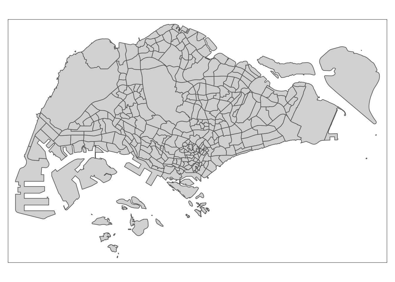
tmap_mode("plot")
tm_shape(mpsz) +
  tm_polygons() +
tm_shape(MRT_Station) +
  tm_dots()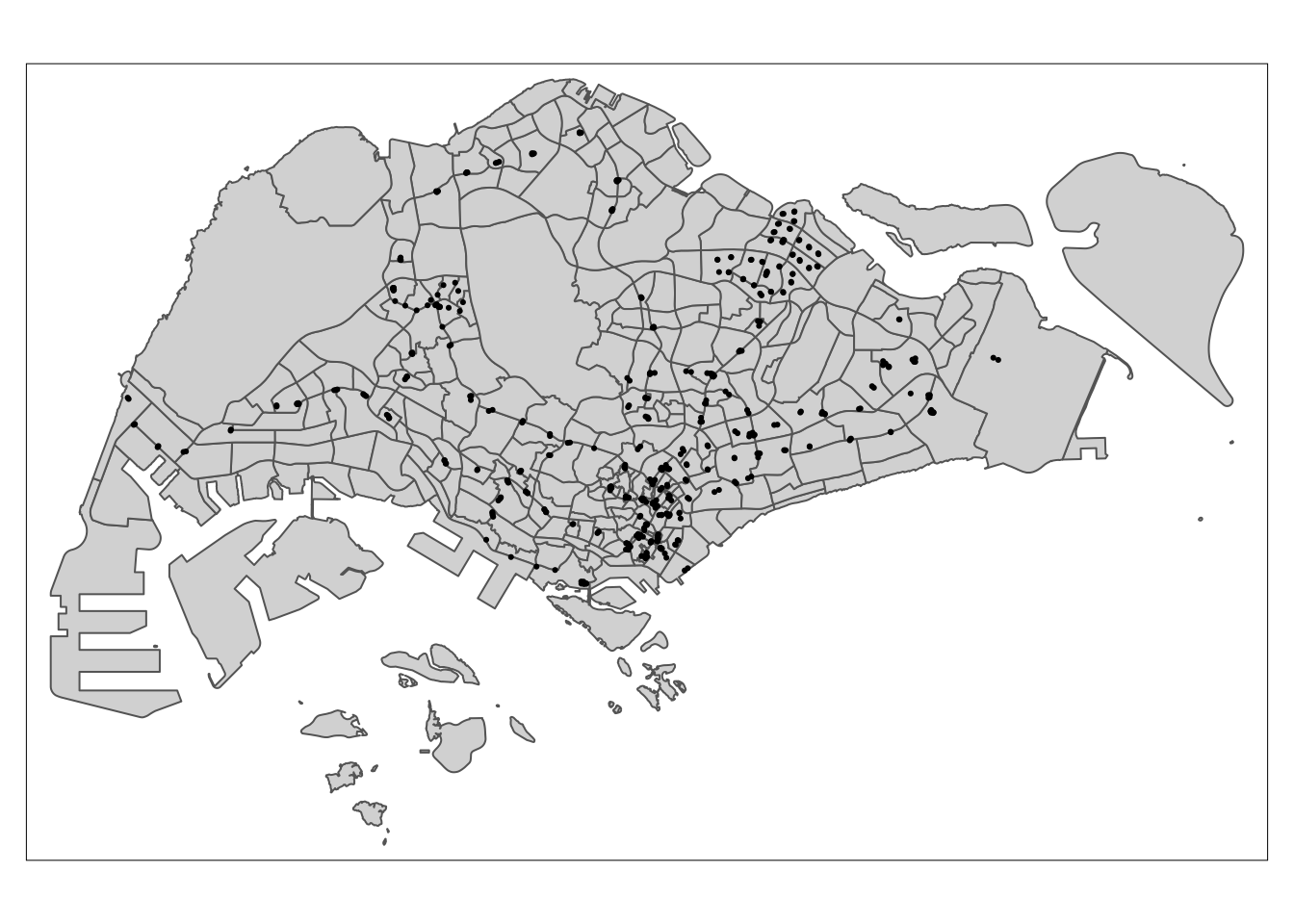
tmap_mode("plot")
tm_shape(mpsz) +
  tm_polygons() +
tm_shape(Bus_stop) +
  tm_dots(col = "red",
          size = 0.0075)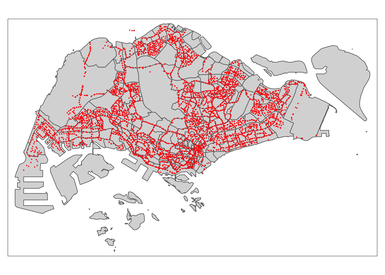
Note that the points outside of Singapore boundaries are related to bus stop at Johor Bahru and they are valid points to our analysis.
tm_shape(mpsz) +
  tm_polygons() +
tm_shape(communityclubs) +
  tm_dots()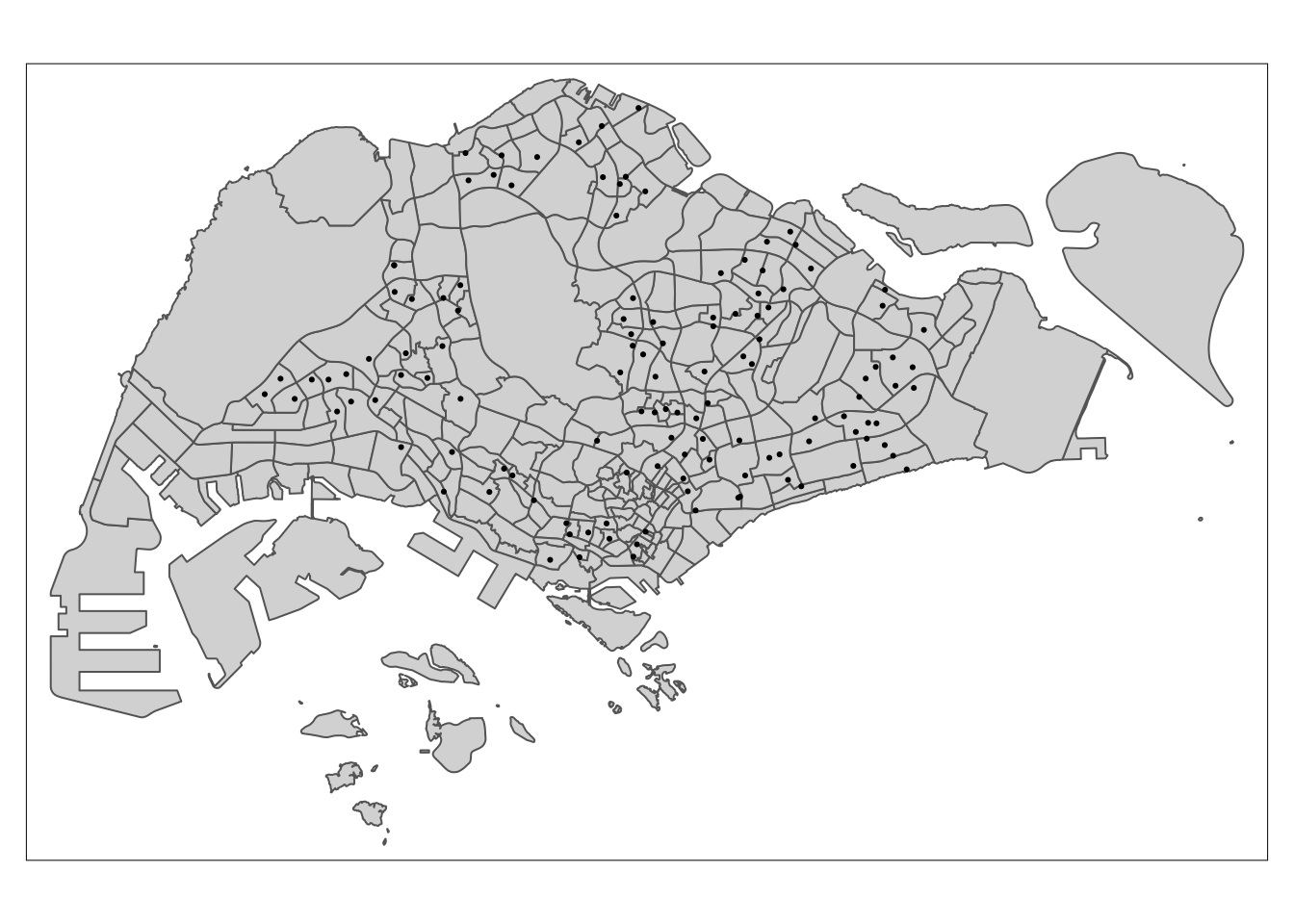
tm_shape(mpsz) +
  tm_polygons() +
tm_shape(eldercare) +
  tm_dots()
tm_shape(mpsz) +
  tm_polygons() +
tm_shape(familyservices) +
  tm_dots()
tm_shape(mpsz) +
  tm_polygons() +
tm_shape(hawker) +
  tm_dots()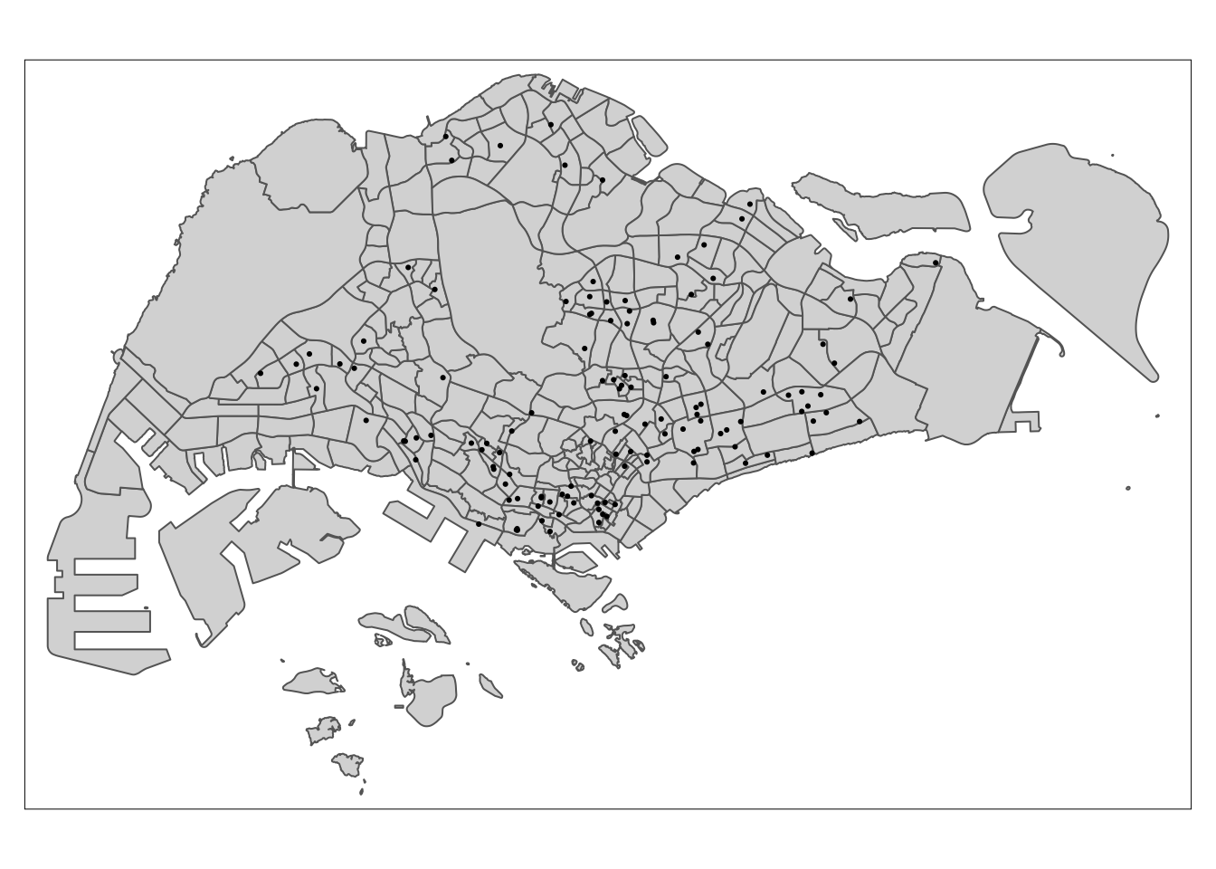
tm_shape(mpsz) +
  tm_polygons() +
tm_shape(kindergartens) +
  tm_dots()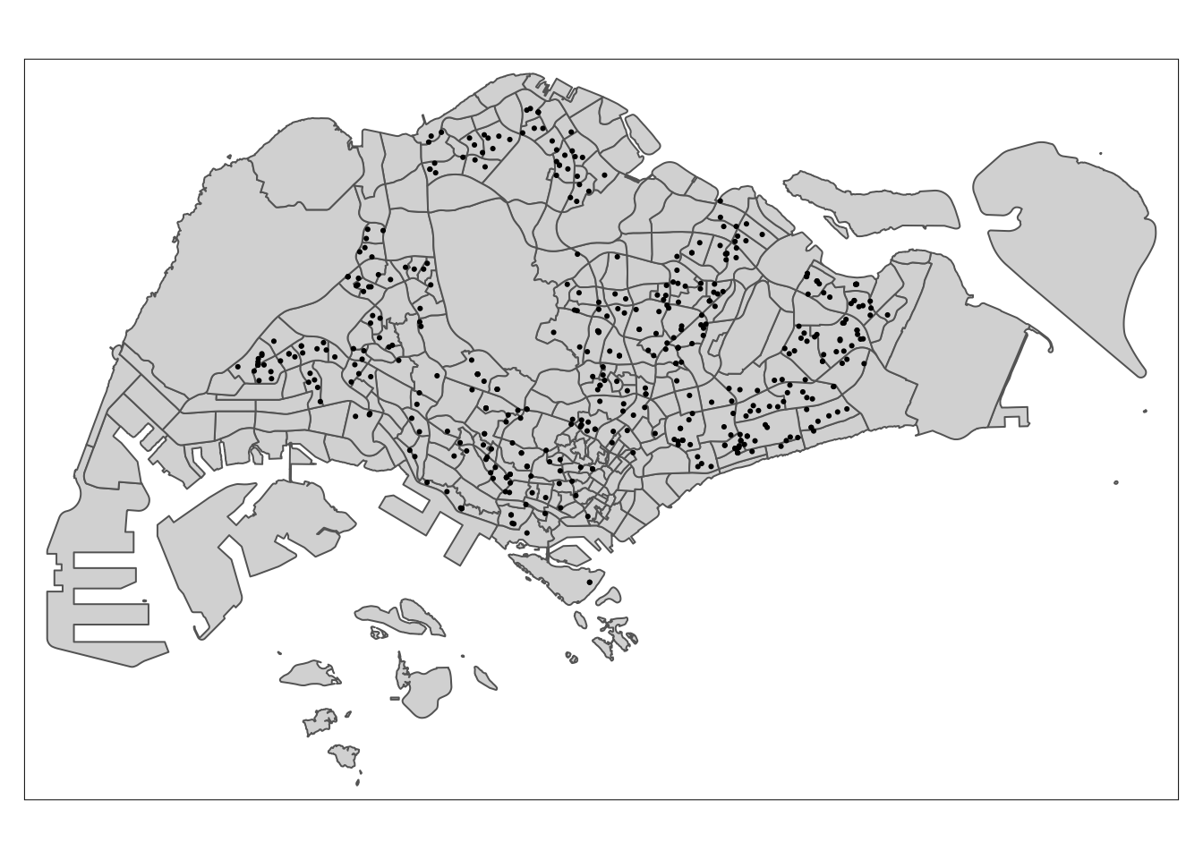
tm_shape(mpsz) +
  tm_polygons() +
tm_shape(malls) +
  tm_dots()
tm_shape(mpsz) +
  tm_polygons() +
tm_shape(parks) +
  tm_dots()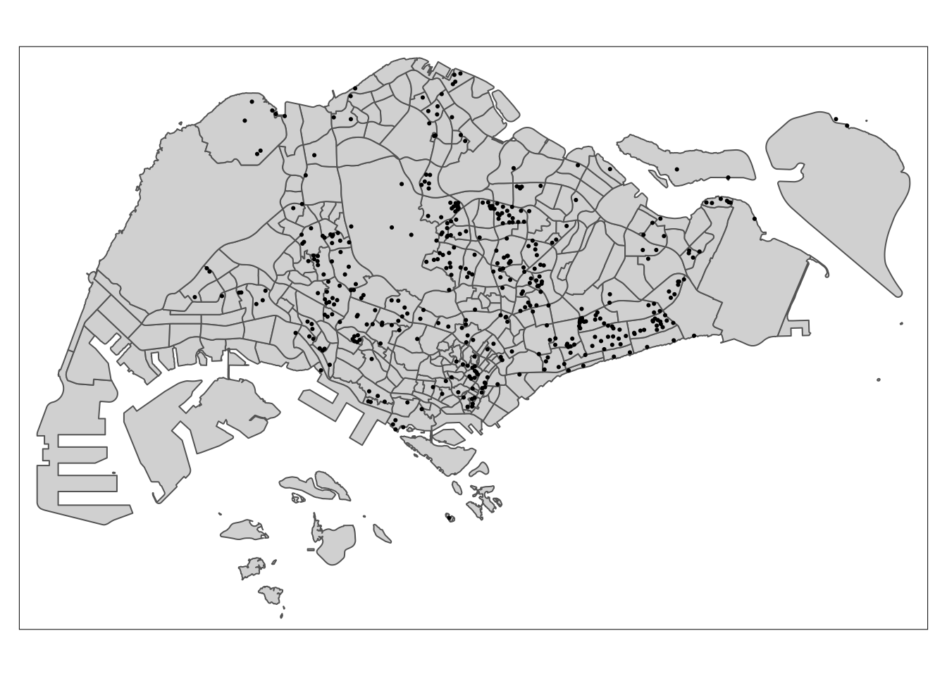
tm_shape(mpsz) +
  tm_polygons() +
tm_shape(pharmacy) +
  tm_dots()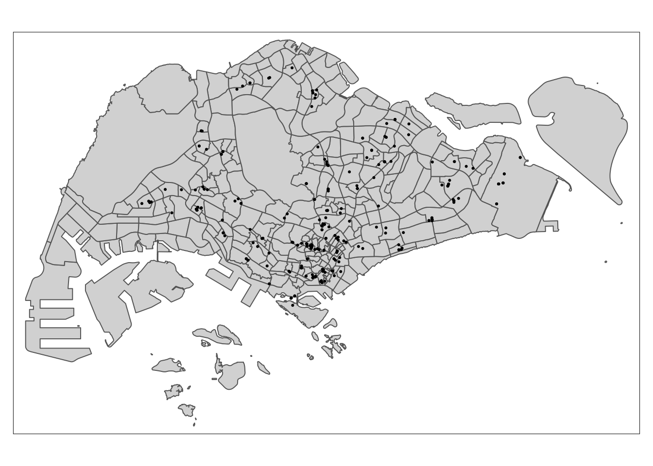
tm_shape(mpsz) +
  tm_polygons() +
tm_shape(childcare) +
  tm_dots()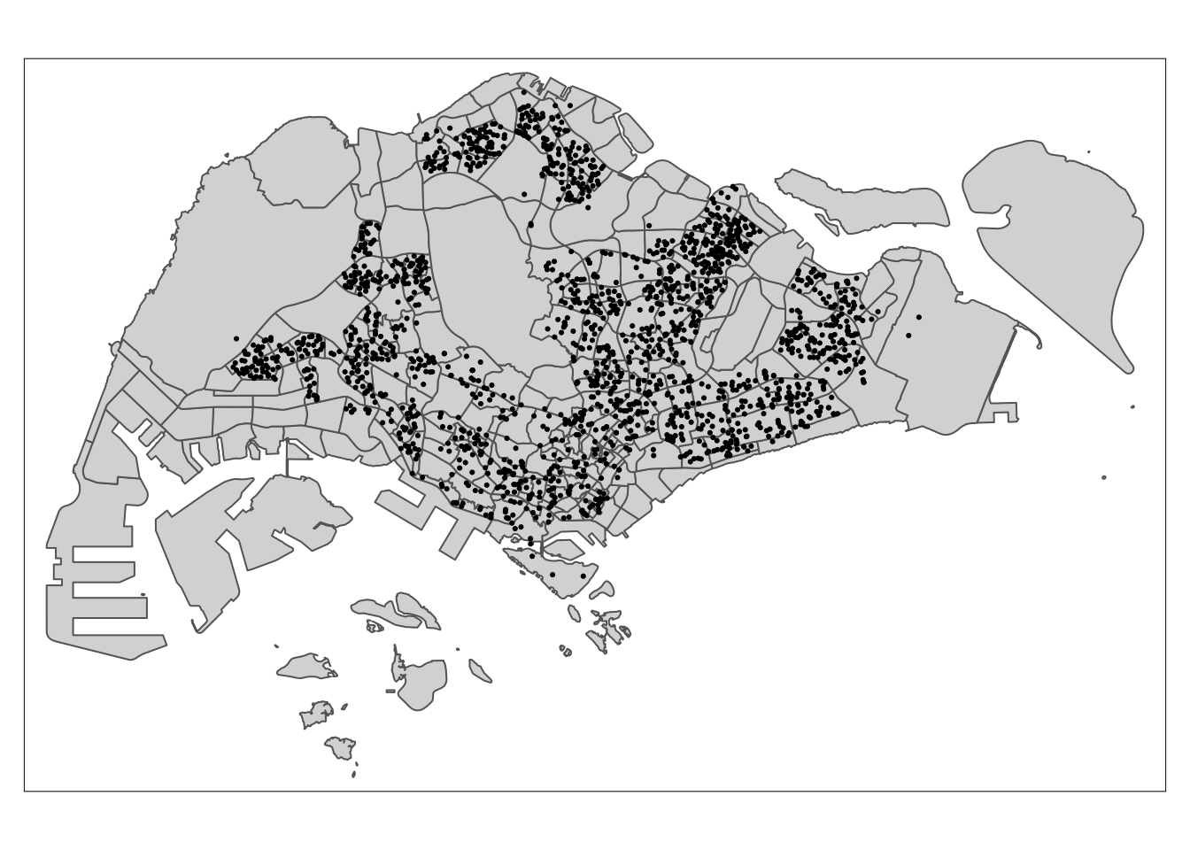
tm_shape(mpsz) +
  tm_polygons() +
tm_shape(Primary_sf) +
  tm_dots()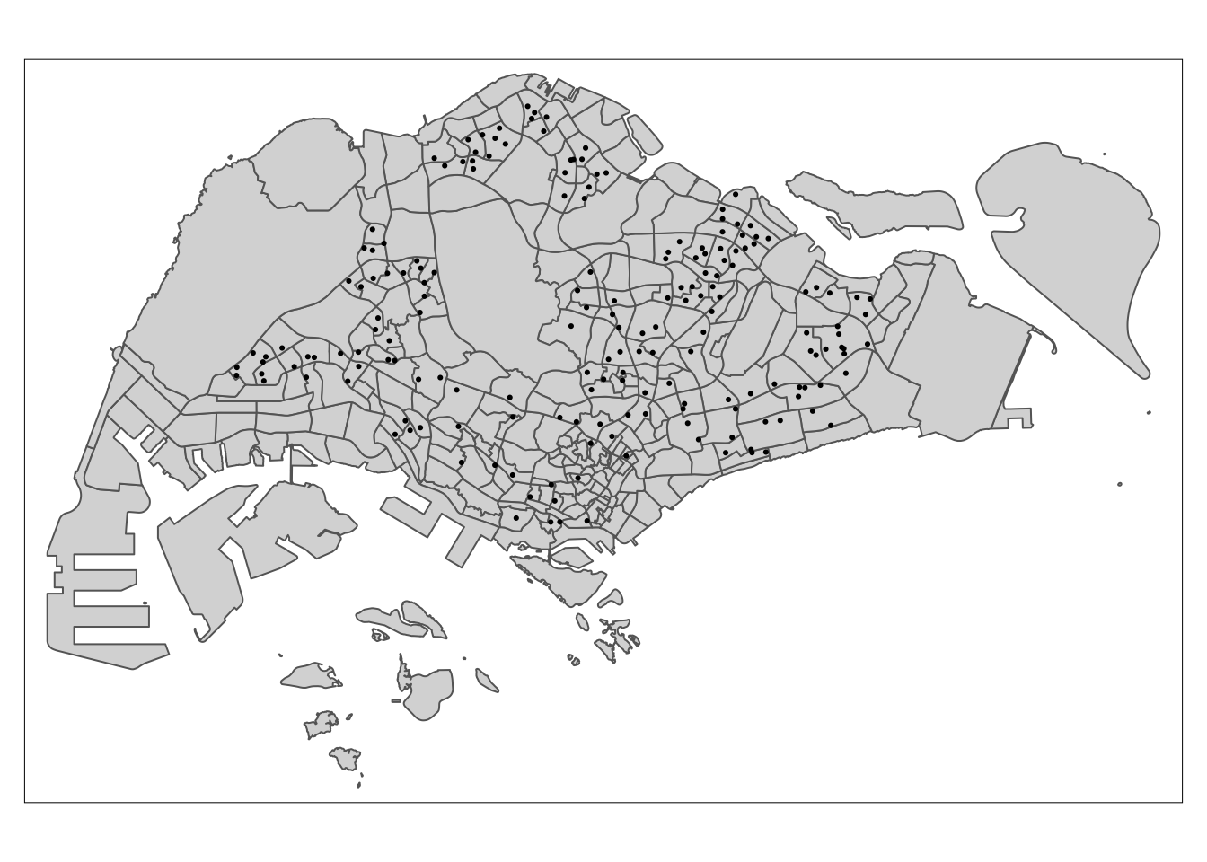
tm_shape(mpsz) +
  tm_polygons() +
tm_shape(Secondary_sf) +
  tm_dots()
5 Proximity distance calculator
Here, we will need to calculate the distance between each variable to the resale apartment.
The code below creates a function called proximity() that takes in 3 values.
library(units)
library(matrixStats)
proximity <- function(df1, df2, varname) {
  dist_matrix <- st_distance(df1, df2) %>%
    drop_units()
  df1[,varname] <- rowMins(dist_matrix)
  return(df1) }
The code chunks in training and test data essentially calculates the proximity between Resale flats and the variable. This is piped each time, creating a new column with the 3rd input name and assigned to the object, training_resale/test_resale.
training_resale <-
  # the columns will be truncated later on when viewing
  # so we're limiting ourselves to two-character columns for ease of viewing between
  proximity(Resale_training_sf, cbd_sf, "PROX_CBD") %>%
  proximity(.,Bus_stop, "PROX_BUS") %>%
  proximity(., communityclubs, "PROX_CLUBS") %>%
  proximity(., eldercare, "PROX_ELDERCARE") %>%
  proximity(., familyservices, "PROX_FAM") %>%
  proximity(., MRT_Station, "PROX_MRT") %>%
  proximity(., hawker, "PROX_HAWKER") %>%
  proximity(., kindergartens, "PROX_KINDERGARTENS") %>%
  proximity(., pharmacy, "PROX_PHARMACY") %>%
  proximity(., parks, "PROX_PARK") %>%
  proximity(., malls, "PROX_MALL") %>%
  proximity(., supermarkets, "PROX_SPRMKT") %>%
  proximity(., childcare, "PROX_CHILDCARE") %>%
  proximity(., Primary_sf, "PROX_PRISCH") %>%
  proximity(., Good_Prisch, "PROX_GOODP") %>%
  proximity(., Secondary_sf, "PROX_SECSCH")
We will change the names of the column for easy recognition and referencing. This is done using mutate() and rename() from the dplyr package
training_resale <- training_resale %>%
  mutate() %>%
  rename("AREA_SQM" = "flr_r_s",
         "PRICE" = "rsl_prc",
         "REMAINING_LEASE" = "rmnng_l") %>%
  relocate(`PRICE`)
test_resale <-
# the columns will be truncated later on when viewing
# so we're limiting ourselves to two-character columns for ease of viewing between
proximity(Resale_test_sf, cbd_sf, "PROX_CBD") %>%
proximity(.,Bus_stop, "PROX_BUS") %>%
proximity(., communityclubs, "PROX_CLUBS") %>%
proximity(., eldercare, "PROX_ELDERCARE") %>%
proximity(., familyservices, "PROX_FAM") %>%
proximity(., MRT_Station, "PROX_MRT") %>%
proximity(., hawker, "PROX_HAWKER") %>%
proximity(., kindergartens, "PROX_KINDERGARTENS") %>%
proximity(., pharmacy, "PROX_PHARMACY") %>%
proximity(., parks, "PROX_PARK") %>%
proximity(., malls, "PROX_MALL") %>%
proximity(., supermarkets, "PROX_SPRMKT") %>%
proximity(., childcare, "PROX_CHILDCARE") %>%
proximity(., Primary_sf, "PROX_PRISCH") %>%
proximity(., Good_Prisch, "PROX_GOODP") %>%
proximity(., Secondary_sf, "PROX_SECSCH") We will change the names of the columns for easy recognition and referencing. This is done using mutate() and rename() from the dplyr package
test_resale <- test_resale %>%
  mutate() %>%
  rename("AREA_SQM" = "flr_r_s",
         "PRICE" = "rsl_prc",
         "REMAINING_LEASE" = "rmnng_l") %>%
  relocate(`PRICE`)
5.1 Facility Count within Radius Calculation
Here, we want to find the number of facilities within a particular radius. Like above, we’ll use st_distance() to compute the distance between the flats and the desired facilities, and then sum up the observations with rowSums(). The values will be appended to the data frame as a new column.
num_radius <- function(df1, df2, varname, radius) {
  dist_matrix <- st_distance(df1, df2) %>%
    drop_units() %>%
    as.data.frame()
  df1[,varname] <- rowSums(dist_matrix <= radius)
  return(df1)
}training_resale <-
num_radius(training_resale, kindergartens, "NUM_KNDRGTN", 350) %>%
num_radius(., childcare, "NUM_CHILDCARE", 350) %>%
num_radius(., Bus_stop, "NUM_BUS_STOP", 350) %>%
num_radius(., Primary_sf, "NUM_PRISCH", 1000) %>%
num_radius(., Secondary_sf, "NUM_SECSCH", 1000)Always make sure to save the object as an rds file for future referencing.
Show code
write_rds(training_resale, "data/aspatial/training_resale.rds")test_resale <-
num_radius(test_resale, kindergartens, "NUM_KNDRGTN", 350) %>%
num_radius(., childcare, "NUM_CHILDCARE", 350) %>%
num_radius(., Bus_stop, "NUM_BUS_STOP", 350) %>%
num_radius(., Primary_sf, "NUM_PRISCH", 1000) %>%
num_radius(., Secondary_sf, "NUM_SECSCH", 1000)Always make sure to save the object as an rds file for future referencing.
write_rds(test_resale, "data/aspatial/test_resale.rds")6 Read Data in
training_data <- read_rds("data/aspatial/training_resale.rds")
test_data <- read_rds("data/aspatial/test_resale.rds")glimpse(training_data)Rows: 14,508
Columns: 50
$ PRICE <dbl> 483000, 590000, 629000, 670000, 680000, 760000, 768…
$ month <date> 2021-01-01, 2021-01-01, 2021-01-01, 2021-01-01, 20…
$ block <chr> "551", "305", "520", "253", "423", "617", "315A", "…
$ strt_nm <chr> "ANG MO KIO AVE 10", "ANG MO KIO AVE 1", "ANG MO KI…
$ AREA_SQM <dbl> 118, 123, 118, 128, 133, 133, 110, 110, 110, 112, 1…
$ REMAINING_LEASE <dbl> 59.08, 55.58, 58.67, 74.25, 71.25, 74.50, 84.33, 80…
$ Stry_Or <dbl> 1, 5, 6, 3, 1, 5, 8, 5, 6, 6, 5, 5, 8, 1, 2, 3, 3, …
$ Improvd <dbl> 1, 0, 1, 1, 1, 0, 1, 1, 1, 0, 0, 0, 0, 0, 1, 1, 1, …
$ NwGnrtn <dbl> 0, 0, 0, 0, 0, 0, 0, 0, 0, 0, 0, 0, 0, 0, 0, 0, 0, …
$ DBSS <dbl> 0, 0, 0, 0, 0, 0, 0, 0, 0, 1, 1, 1, 1, 0, 0, 0, 0, …
$ Standrd <dbl> 0, 1, 0, 0, 0, 0, 0, 0, 0, 0, 0, 0, 0, 1, 0, 0, 0, …
$ Aprtmnt <dbl> 0, 0, 0, 0, 0, 0, 0, 0, 0, 0, 0, 0, 0, 0, 0, 0, 0, …
$ Simplfd <dbl> 0, 0, 0, 0, 0, 0, 0, 0, 0, 0, 0, 0, 0, 0, 0, 0, 0, …
$ Model.A <dbl> 0, 0, 0, 0, 0, 1, 0, 0, 0, 0, 0, 0, 0, 0, 0, 0, 0, …
$ PrmmApr <dbl> 0, 0, 0, 0, 0, 0, 0, 0, 0, 0, 0, 0, 0, 0, 0, 0, 0, …
$ Adjndfl <dbl> 0, 0, 0, 0, 0, 0, 0, 0, 0, 0, 0, 0, 0, 0, 0, 0, 0, …
$ MdlA.Ms <dbl> 0, 0, 0, 0, 0, 0, 0, 0, 0, 0, 0, 0, 0, 0, 0, 0, 0, …
$ Maisntt <dbl> 0, 0, 0, 0, 0, 0, 0, 0, 0, 0, 0, 0, 0, 0, 0, 0, 0, …
$ Type.S1 <dbl> 0, 0, 0, 0, 0, 0, 0, 0, 0, 0, 0, 0, 0, 0, 0, 0, 0, …
$ Type.S2 <dbl> 0, 0, 0, 0, 0, 0, 0, 0, 0, 0, 0, 0, 0, 0, 0, 0, 0, …
$ ModelA2 <dbl> 0, 0, 0, 0, 0, 0, 0, 0, 0, 0, 0, 0, 0, 0, 0, 0, 0, …
$ Terrace <dbl> 0, 0, 0, 0, 0, 0, 0, 0, 0, 0, 0, 0, 0, 0, 0, 0, 0, …
$ Imprv.M <dbl> 0, 0, 0, 0, 0, 0, 0, 0, 0, 0, 0, 0, 0, 0, 0, 0, 0, …
$ PrmmMsn <dbl> 0, 0, 0, 0, 0, 0, 0, 0, 0, 0, 0, 0, 0, 0, 0, 0, 0, …
$ MltGnrt <dbl> 0, 0, 0, 0, 0, 0, 0, 0, 0, 0, 0, 0, 0, 0, 0, 0, 0, …
$ PrmmApL <dbl> 0, 0, 0, 0, 0, 0, 0, 0, 0, 0, 0, 0, 0, 0, 0, 0, 0, …
$ X2.room <dbl> 0, 0, 0, 0, 0, 0, 0, 0, 0, 0, 0, 0, 0, 0, 0, 0, 0, …
$ X3Gen <dbl> 0, 0, 0, 0, 0, 0, 0, 0, 0, 0, 0, 0, 0, 0, 0, 0, 0, …
$ PROX_CBD <dbl> 9537.543, 8663.223, 9449.166, 9211.988, 8935.289, 1…
$ PROX_BUS <dbl> 189.45342, 199.24454, 80.68454, 160.52022, 91.01582…
$ PROX_CLUBS <dbl> 1039.74076, 600.65527, 250.17807, 511.71420, 414.13…
$ PROX_ELDERCARE <dbl> 1064.6617, 190.8834, 789.1907, 147.6040, 441.8627, …
$ PROX_FAM <dbl> 837.9872, 953.8865, 863.1507, 366.4593, 466.4299, 9…
$ PROX_MRT <dbl> 1080.8607, 524.3923, 415.9309, 1634.1785, 218.2533,…
$ PROX_HAWKER <dbl> 482.8156, 331.7637, 379.2242, 588.4497, 512.9672, 3…
$ PROX_KINDERGARTENS <dbl> 239.51930, 148.29403, 224.35730, 270.32452, 295.950…
$ PROX_PHARMACY <dbl> 1254.2522, 439.1980, 455.9529, 1331.3597, 379.1169,…
$ PROX_PARK <dbl> 735.9373, 580.8933, 308.7999, 283.8337, 257.6041, 3…
$ PROX_MALL <dbl> 1213.2871, 441.6229, 549.4572, 1536.9839, 371.1503,…
$ PROX_SPRMKT <dbl> 419.91387, 245.54343, 318.05791, 313.57577, 379.115…
$ PROX_CHILDCARE <dbl> 239.51930, 111.38938, 127.59057, 102.48186, 288.529…
$ PROX_PRISCH <dbl> 809.7020, 558.0558, 213.5757, 567.7924, 312.2025, 2…
$ PROX_GOODP <dbl> 5849.176, 5370.382, 6221.695, 5429.407, 5759.906, 6…
$ PROX_SECSCH <dbl> 792.7406, 451.2317, 113.4179, 152.8092, 317.5082, 4…
$ geometry <POINT [m]> POINT (30820.82 39547.58), POINT (29412.84 38…
$ NUM_KNDRGTN <dbl> 1, 1, 1, 1, 1, 1, 1, 0, 1, 1, 1, 1, 1, 0, 0, 1, 0, …
$ NUM_CHILDCARE <dbl> 3, 6, 4, 3, 3, 3, 5, 2, 6, 5, 6, 5, 5, 2, 4, 3, 2, …
$ NUM_BUS_STOP <dbl> 2, 8, 6, 11, 6, 8, 4, 9, 5, 9, 7, 9, 9, 7, 6, 5, 2,…
$ NUM_PRISCH <dbl> 1, 3, 2, 3, 3, 3, 4, 2, 2, 2, 2, 2, 2, 3, 2, 1, 3, …
$ NUM_SECSCH <dbl> 1, 2, 2, 3, 2, 2, 2, 2, 2, 2, 2, 2, 2, 4, 0, 1, 1, …We can see that we have forgotten to remove Block and street. We can also check and confirm that all variables are in the right format.
training_data <- training_data %>%
select(-block, -strt_nm)glimpse(test_data)Rows: 998
Columns: 50
$ PRICE <dbl> 682888.0, 695000.0, 658888.0, 748000.0, 790000.0, 7…
$ month <date> 2023-01-01, 2023-01-01, 2023-01-01, 2023-02-01, 20…
$ block <chr> "306", "306", "402", "431", "259", "259", "176", "6…
$ strt_nm <chr> "ANG MO KIO AVE 1", "ANG MO KIO AVE 1", "ANG MO KIO…
$ AREA_SQM <dbl> 123, 123, 119, 119, 135, 135, 119, 133, 135, 118, 1…
$ REMAINING_LEASE <dbl> 53.58, 53.58, 55.42, 54.92, 58.42, 58.17, 69.33, 72…
$ Stry_Or <dbl> 6, 2, 4, 8, 5, 1, 2, 5, 4, 7, 7, 4, 2, 3, 3, 1, 2, …
$ Improvd <dbl> 0, 0, 1, 1, 0, 0, 1, 0, 0, 1, 1, 1, 1, 0, 0, 1, 1, …
$ NwGnrtn <dbl> 0, 0, 0, 0, 0, 0, 0, 0, 0, 0, 0, 0, 0, 0, 0, 0, 0, …
$ DBSS <dbl> 0, 0, 0, 0, 0, 0, 0, 0, 0, 0, 0, 0, 0, 0, 0, 0, 0, …
$ Standrd <dbl> 1, 1, 0, 0, 0, 0, 0, 0, 0, 0, 0, 0, 0, 0, 0, 0, 0, …
$ Aprtmnt <dbl> 0, 0, 0, 0, 0, 0, 0, 0, 0, 0, 0, 0, 0, 0, 0, 0, 0, …
$ Simplfd <dbl> 0, 0, 0, 0, 0, 0, 0, 0, 0, 0, 0, 0, 0, 0, 0, 0, 0, …
$ Model.A <dbl> 0, 0, 0, 0, 1, 1, 0, 1, 1, 0, 0, 0, 0, 1, 1, 0, 0, …
$ PrmmApr <dbl> 0, 0, 0, 0, 0, 0, 0, 0, 0, 0, 0, 0, 0, 0, 0, 0, 0, …
$ Adjndfl <dbl> 0, 0, 0, 0, 0, 0, 0, 0, 0, 0, 0, 0, 0, 0, 0, 0, 0, …
$ MdlA.Ms <dbl> 0, 0, 0, 0, 0, 0, 0, 0, 0, 0, 0, 0, 0, 0, 0, 0, 0, …
$ Maisntt <dbl> 0, 0, 0, 0, 0, 0, 0, 0, 0, 0, 0, 0, 0, 0, 0, 0, 0, …
$ Type.S1 <dbl> 0, 0, 0, 0, 0, 0, 0, 0, 0, 0, 0, 0, 0, 0, 0, 0, 0, …
$ Type.S2 <dbl> 0, 0, 0, 0, 0, 0, 0, 0, 0, 0, 0, 0, 0, 0, 0, 0, 0, …
$ ModelA2 <dbl> 0, 0, 0, 0, 0, 0, 0, 0, 0, 0, 0, 0, 0, 0, 0, 0, 0, …
$ Terrace <dbl> 0, 0, 0, 0, 0, 0, 0, 0, 0, 0, 0, 0, 0, 0, 0, 0, 0, …
$ Imprv.M <dbl> 0, 0, 0, 0, 0, 0, 0, 0, 0, 0, 0, 0, 0, 0, 0, 0, 0, …
$ PrmmMsn <dbl> 0, 0, 0, 0, 0, 0, 0, 0, 0, 0, 0, 0, 0, 0, 0, 0, 0, …
$ MltGnrt <dbl> 0, 0, 0, 0, 0, 0, 0, 0, 0, 0, 0, 0, 0, 0, 0, 0, 0, …
$ PrmmApL <dbl> 0, 0, 0, 0, 0, 0, 0, 0, 0, 0, 0, 0, 0, 0, 0, 0, 0, …
$ X2.room <dbl> 0, 0, 0, 0, 0, 0, 0, 0, 0, 0, 0, 0, 0, 0, 0, 0, 0, …
$ X3Gen <dbl> 0, 0, 0, 0, 0, 0, 0, 0, 0, 0, 0, 0, 0, 0, 0, 0, 0, …
$ PROX_CBD <dbl> 8625.861, 8625.861, 8139.329, 8876.533, 9195.256, 9…
$ PROX_BUS <dbl> 178.81652, 178.81652, 118.76102, 197.29080, 84.2301…
$ PROX_CLUBS <dbl> 578.73029, 578.73029, 265.15993, 546.71811, 832.788…
$ PROX_ELDERCARE <dbl> 211.9637, 211.9637, 367.6850, 356.4709, 501.9017, 5…
$ PROX_FAM <dbl> 940.0572, 940.0572, 612.9699, 319.3456, 706.0581, 7…
$ PROX_MRT <dbl> 573.2417, 573.2417, 1065.8815, 365.2200, 1981.5890,…
$ PROX_HAWKER <dbl> 331.2628, 331.2628, 143.0536, 375.3304, 508.2023, 5…
$ PROX_KINDERGARTENS <dbl> 188.26098, 188.26098, 518.63595, 148.88003, 450.529…
$ PROX_PHARMACY <dbl> 488.5421, 488.5421, 1152.5507, 522.2008, 1540.0063,…
$ PROX_PARK <dbl> 554.3174, 554.3174, 537.1188, 390.1731, 294.0396, 2…
$ PROX_MALL <dbl> 490.9497, 490.9497, 1145.3444, 514.1228, 1582.3113,…
$ PROX_SPRMKT <dbl> 246.50070, 246.50070, 504.07157, 313.59260, 541.623…
$ PROX_CHILDCARE <dbl> 1.580294e+02, 1.580294e+02, 3.274622e+02, 1.488800e…
$ PROX_PRISCH <dbl> 585.34956, 585.34956, 240.18714, 358.85813, 899.237…
$ PROX_GOODP <dbl> 5325.218, 5325.218, 4880.120, 5632.979, 5155.426, 5…
$ PROX_SECSCH <dbl> 438.0324, 438.0324, 586.3205, 250.5094, 259.7381, 2…
$ geometry <POINT [m]> POINT (29383.53 38640.51), POINT (29383.53 38…
$ NUM_KNDRGTN <dbl> 1, 1, 0, 1, 0, 0, 1, 0, 0, 1, 2, 1, 1, 1, 1, 1, 1, …
$ NUM_CHILDCARE <dbl> 6, 6, 1, 4, 2, 2, 3, 5, 5, 4, 8, 4, 3, 3, 2, 6, 3, …
$ NUM_BUS_STOP <dbl> 6, 6, 7, 6, 6, 6, 6, 8, 10, 6, 8, 10, 11, 11, 10, 5…
$ NUM_PRISCH <dbl> 3, 3, 2, 3, 3, 3, 2, 2, 2, 2, 3, 3, 3, 3, 2, 2, 3, …
$ NUM_SECSCH <dbl> 2, 2, 1, 2, 2, 2, 3, 2, 2, 2, 3, 4, 3, 3, 3, 2, 1, …We can see that we have forgotten to remove Block and street. We can also check and confirm that all variables are in the right format.
test_data <- test_data %>%
  select(-block, -strt_nm)
7 Computing Correlation Matrix
training_data_nogeo <- training_data %>%
  st_drop_geometry()
We will first create the correlation matrix and check for any NA or infinite values.
cor_matrix <- cor(training_data_nogeo[,3:47])
any(is.na(cor_matrix)) # check for missing values
[1] TRUEany(is.infinite(cor_matrix)) # check for infinite values[1] FALSESince there are missing values, we will fix this by assigning 0 to them
na_value <- is.na(cor_matrix)
cor_matrix[na_value] <- 0corrplot::corrplot(cor_matrix,
diag = FALSE,
order = "AOE",
tl.pos = "td",
tl.cex = 0.2,
method = "number",
type = "upper")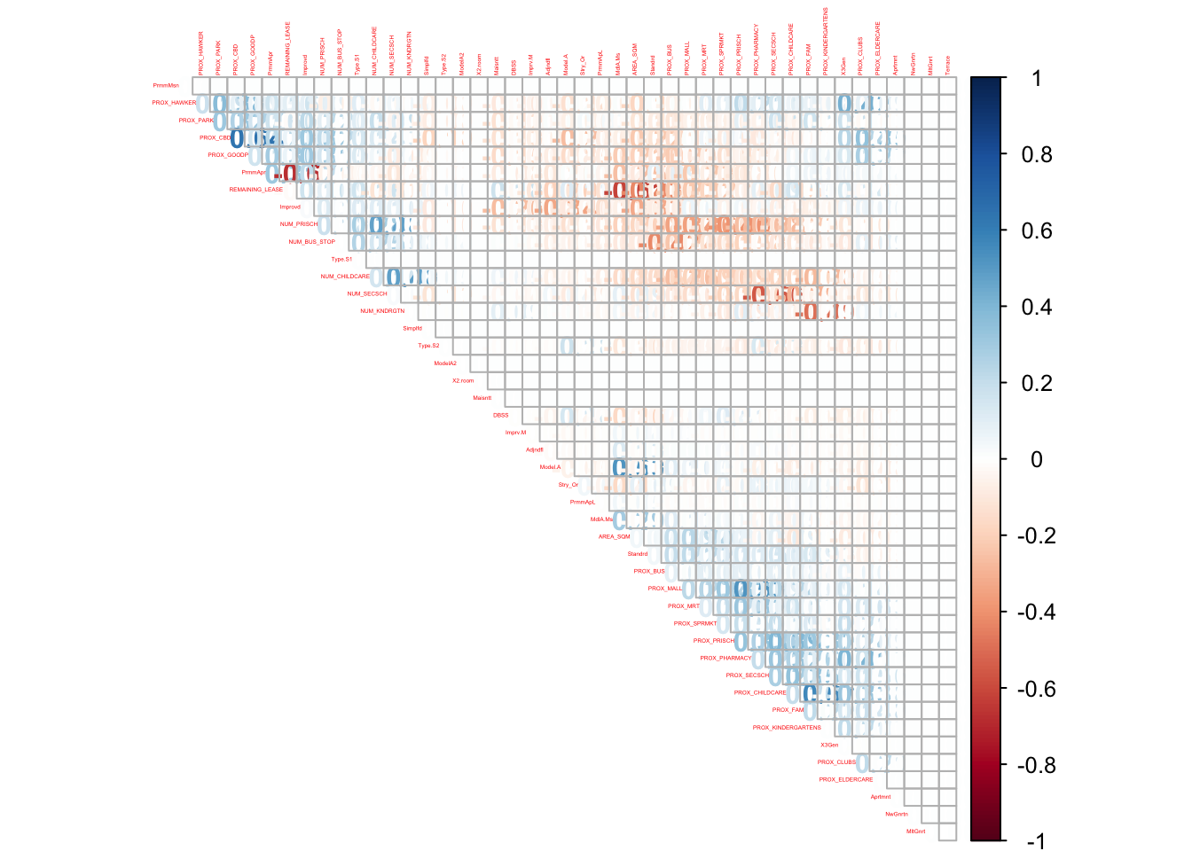
We can see several correlated variables above 0.5 but they are within acceptable range to be included in the regression. However, it would be better to remove PROX_KINDERGARTENS, PROX_CHILDCARE, PROX_BUS, PROX_PRISCH and PROX_SECSCH. This is because the effects from these 5 variables would have been captured in the facility count, NUM_ . While the correlation matrix suggest no high correlation, it could create bias in our estimator should the variables be correlated.
8 Building a non-spatial multiple linear regression
We will run the multiple linear regression using the base R function, lm().
price_mlr1 <- lm(PRICE ~ AREA_SQM + REMAINING_LEASE + Stry_Or + Improvd + DBSS + Standrd + Model.A + PrmmApr + Adjndfl + MdlA.Ms + Type.S2 + Imprv.M + PrmmApL + PROX_CBD + PROX_CLUBS + PROX_ELDERCARE + PROX_FAM + PROX_MRT +PROX_HAWKER + PROX_PHARMACY +PROX_PARK+PROX_MALL + PROX_SPRMKT + PROX_GOODP + NUM_KNDRGTN + NUM_CHILDCARE + NUM_BUS_STOP + NUM_PRISCH + NUM_SECSCH,
                data = training_data)
We can first save the model by running the code chunk below.
Show code
write_rds(price_mlr1, "data/model/price_mlr1.rds")price_mlr1 <- read_rds("data/model/price_mlr1.rds")8.1 Understanding the non-spatial multiple linear regression model
summary(price_mlr1)
Call:
lm(formula = PRICE ~ AREA_SQM + REMAINING_LEASE + Stry_Or + Improvd +
    DBSS + Standrd + Model.A + PrmmApr + Adjndfl + MdlA.Ms +
    Type.S2 + Imprv.M + PrmmApL + PROX_CBD + PROX_CLUBS + PROX_ELDERCARE +
    PROX_FAM + PROX_MRT + PROX_HAWKER + PROX_PHARMACY + PROX_PARK +
    PROX_MALL + PROX_SPRMKT + PROX_GOODP + NUM_KNDRGTN + NUM_CHILDCARE +
    NUM_BUS_STOP + NUM_PRISCH + NUM_SECSCH, data = training_data)

Residuals:
    Min      1Q  Median      3Q     Max
-259902  -50073   -2595   45960  697099

Coefficients:
                  Estimate Std. Error t value Pr(>|t|)
(Intercept)     -3.188e+05  4.201e+04  -7.589 3.41e-14 ***
AREA_SQM         6.767e+03  1.547e+02  43.734  < 2e-16 ***
REMAINING_LEASE  5.948e+03  9.011e+01  66.007  < 2e-16 ***
Stry_Or          1.818e+04  3.270e+02  55.610  < 2e-16 ***
Improvd         -1.097e+04  3.426e+04  -0.320 0.748883
DBSS             1.460e+05  3.447e+04   4.236 2.29e-05 ***
Standrd          4.393e+04  3.451e+04   1.273 0.203118
Model.A         -4.312e+04  3.438e+04  -1.254 0.209755
PrmmApr         -5.752e+03  3.428e+04  -0.168 0.866730
Adjndfl         -1.602e+04  3.622e+04  -0.442 0.658292
MdlA.Ms          1.366e+04  3.502e+04   0.390 0.696473
Type.S2          1.642e+05  3.571e+04   4.598 4.30e-06 ***
Imprv.M          9.382e+03  4.841e+04   0.194 0.846324
PrmmApL          1.838e+05  4.367e+04   4.208 2.59e-05 ***
PROX_CBD        -1.948e+01  2.567e-01 -75.884  < 2e-16 ***
PROX_CLUBS       2.202e+01  2.801e+00   7.860 4.10e-15 ***
PROX_ELDERCARE   5.401e+00  1.143e+00   4.726 2.31e-06 ***
PROX_FAM        -3.407e+01  1.396e+00 -24.397  < 2e-16 ***
PROX_MRT        -9.855e+00  1.898e+00  -5.193 2.09e-07 ***
PROX_HAWKER     -2.967e+01  1.417e+00 -20.946  < 2e-16 ***
PROX_PHARMACY   -8.325e+00  2.463e+00  -3.380 0.000728 ***
PROX_PARK        1.550e+01  1.666e+00   9.301  < 2e-16 ***
PROX_MALL       -2.494e+01  2.236e+00 -11.152  < 2e-16 ***
PROX_SPRMKT     -2.795e+01  4.367e+00  -6.400 1.61e-10 ***
PROX_GOODP      -4.158e-01  2.891e-01  -1.438 0.150363
NUM_KNDRGTN      1.060e+04  7.090e+02  14.949  < 2e-16 ***
NUM_CHILDCARE   -5.565e+03  3.491e+02 -15.940  < 2e-16 ***
NUM_BUS_STOP    -1.417e+02  2.304e+02  -0.615 0.538627
NUM_PRISCH      -1.068e+04  5.255e+02 -20.319  < 2e-16 ***
NUM_SECSCH      -2.021e+03  6.474e+02  -3.122 0.001798 **
---
Signif. codes:  0 '***' 0.001 '**' 0.01 '*' 0.05 '.' 0.1 ' ' 1

Residual standard error: 76410 on 14478 degrees of freedom
Multiple R-squared:  0.7271,    Adjusted R-squared:  0.7266
F-statistic:  1330 on 29 and 14478 DF,  p-value: < 2.2e-16
We can visualise the regression as a table by using gtsummary package.
gtsummary::tbl_regression(price_mlr1)| Characteristic | Beta | 95% CI1 | p-value |
|---|---|---|---|
| AREA_SQM | 6,767 | 6,464, 7,071 | <0.001 |
| REMAINING_LEASE | 5,948 | 5,771, 6,125 | <0.001 |
| Stry_Or | 18,183 | 17,542, 18,824 | <0.001 |
| Improvd | -10,966 | -78,114, 56,182 | 0.7 |
| DBSS | 146,011 | 78,446, 213,575 | <0.001 |
| Standrd | 43,929 | -23,724, 111,582 | 0.2 |
| Model.A | -43,118 | -110,500, 24,264 | 0.2 |
| PrmmApr | -5,752 | -72,940, 61,435 | 0.9 |
| Adjndfl | -16,019 | -87,011, 54,974 | 0.7 |
| MdlA.Ms | 13,661 | -54,984, 82,307 | 0.7 |
| Type.S2 | 164,201 | 94,207, 234,196 | <0.001 |
| Imprv.M | 9,382 | -85,505, 104,270 | 0.8 |
| PrmmApL | 183,756 | 98,165, 269,348 | <0.001 |
| PROX_CBD | -19 | -20, -19 | <0.001 |
| PROX_CLUBS | 22 | 17, 28 | <0.001 |
| PROX_ELDERCARE | 5.4 | 3.2, 7.6 | <0.001 |
| PROX_FAM | -34 | -37, -31 | <0.001 |
| PROX_MRT | -9.9 | -14, -6.1 | <0.001 |
| PROX_HAWKER | -30 | -32, -27 | <0.001 |
| PROX_PHARMACY | -8.3 | -13, -3.5 | <0.001 |
| PROX_PARK | 15 | 12, 19 | <0.001 |
| PROX_MALL | -25 | -29, -21 | <0.001 |
| PROX_SPRMKT | -28 | -37, -19 | <0.001 |
| PROX_GOODP | -0.42 | -0.98, 0.15 | 0.2 |
| NUM_KNDRGTN | 10,599 | 9,209, 11,989 | <0.001 |
| NUM_CHILDCARE | -5,565 | -6,249, -4,881 | <0.001 |
| NUM_BUS_STOP | -142 | -593, 310 | 0.5 |
| NUM_PRISCH | -10,677 | -11,707, -9,647 | <0.001 |
| NUM_SECSCH | -2,021 | -3,290, -752 | 0.002 |
| 1 CI = Confidence Interval | |||
From the multiple linear regression model above, we notice that adjusted R square is at 0.7266. This suggest that the model can explain 0.7266 of the variation in Resale Price. We also notice that majority of the proximity variables are significant at the 1% level. This can also be said for AREASQM, REMAINING LEASE AND STORY OR. The model of the apartment did not have significant impact on the Resale Price. However, two model type, DBSS and Type.S2 are significant.
8.2 Calculating predictive error
lm_predicted_value <- predict.lm(price_mlr1, newdata = test_data)

# Calculate MSE
MSE <- mean((test_data$PRICE - lm_predicted_value)^2)

rmse_lm <- sqrt(MSE)
rmse_lm
[1] 87822.93From the square-root of the mean square error is 87822.93. We will take note of this value in the later parts of the regression modelling.
We can compare models using Akaike information criterion (AIC). The smaller the AIC, the better the model. We will find the AIC by running the code chunk below.
AIC(price_mlr1)[1] 367455.5We will just take note of this number and move along with the other models.
9 GWR Predictive Method
9.1 Converting sf dataframe to SpatialPointDataframe
First, we will need to change the training dataframe into a Spatial point data frame. This is used to calculate the other sections in this portion of the Exercise.
train_data_sp <- as_Spatial(training_data)
train_data_sp
class : SpatialPointsDataFrame
features : 14508
extent : 6958.193, 42645.18, 28157.26, 48741.06 (xmin, xmax, ymin, ymax)
crs : +proj=tmerc +lat_0=1.36666666666667 +lon_0=103.833333333333 +k=1 +x_0=28001.642 +y_0=38744.572 +ellps=WGS84 +towgs84=0,0,0,0,0,0,0 +units=m +no_defs
variables : 47
names : PRICE, month, AREA_SQM, REMAINING_LEASE, Stry_Or, Improvd, NwGnrtn, DBSS, Standrd, Aprtmnt, Simplfd, Model.A, PrmmApr, Adjndfl, MdlA.Ms, ...
min values : 350000, 18628, 99, 49.08, 1, 0, 0, 0, 0, 0, 0, 0, 0, 0, 0, ...
max values : 1418000, 19327, 167, 96.75, 17, 1, 0, 1, 1, 0, 0, 1, 1, 1, 1, ... 9.2 Finding optimal adaptive bandwidth
We will find the optimal adaptive bandwidth of the geospatial weighted regression. The code chunk below uses bw.gwr() from the GWModel package:
bw_adaptive <- bw.gwr(PRICE ~ AREA_SQM + REMAINING_LEASE + Stry_Or + Improvd + DBSS + Standrd + Model.A + PrmmApr + Adjndfl + MdlA.Ms + Type.S2 + Imprv.M + PrmmApL + PROX_CBD + PROX_CLUBS + PROX_ELDERCARE + PROX_FAM + PROX_MRT +PROX_HAWKER + PROX_PHARMACY +PROX_PARK+PROX_MALL + PROX_SPRMKT + PROX_GOODP + NUM_KNDRGTN + NUM_CHILDCARE + NUM_BUS_STOP + NUM_PRISCH + NUM_SECSCH,
                data = train_data_sp,
                  approach="CV",
                  kernel="gaussian",
                  adaptive=TRUE,
                  longlat=FALSE)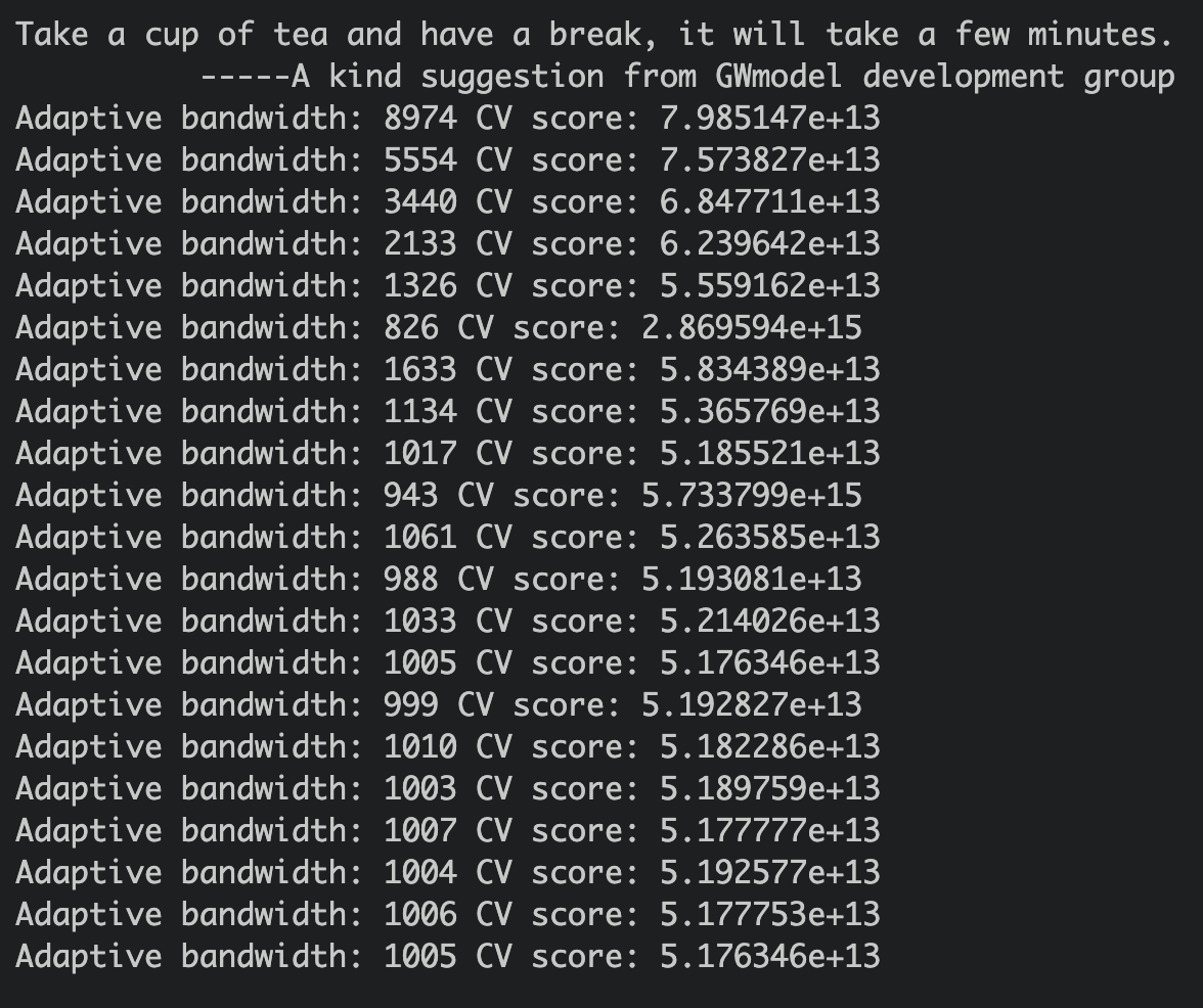
The smallest CV score is adaptive bandwidth: 1005.
We will save the adaptive bandwidth as an RDS file for easy retrieval.
write_rds(bw_adaptive, file = "data/model/bw_adaptive.rds")9.3 Constructing the adaptive bandwidth GWR
We will retrieve the adaptive bandwidth by using read_rds from the readr package.
bw_adaptive <- read_rds("data/model/bw_adaptive.rds")
bw_adaptive
[1] 1005gwr_adaptive <- gwr.basic(formula = PRICE ~ AREA_SQM + REMAINING_LEASE + Stry_Or + Improvd + DBSS + Standrd + Model.A + PrmmApr + Adjndfl + MdlA.Ms + Type.S2 + Imprv.M + PrmmApL + PROX_CBD + PROX_CLUBS + PROX_ELDERCARE + PROX_FAM + PROX_MRT +PROX_HAWKER + PROX_PHARMACY +PROX_PARK+PROX_MALL + PROX_SPRMKT + PROX_GOODP + NUM_KNDRGTN + NUM_CHILDCARE + NUM_BUS_STOP + NUM_PRISCH + NUM_SECSCH,
data = train_data_sp,
bw=bw_adaptive,
kernel = 'gaussian',
adaptive=TRUE,
longlat = FALSE)Again we will save the the regression model as an rds file.
write_rds(gwr_adaptive, "data/model/gwr_adaptive.rds")gwr_adaptive <- read_rds("data/model/gwr_adaptive.rds")
gwr_adaptive ***********************************************************************
* Package GWmodel *
***********************************************************************
Program starts at: 2023-03-17 12:49:34
Call:
gwr.basic(formula = PRICE ~ AREA_SQM + REMAINING_LEASE + Stry_Or +
Improvd + DBSS + Standrd + Model.A + PrmmApr + Adjndfl +
MdlA.Ms + Type.S2 + Imprv.M + PrmmApL + PROX_CBD + PROX_CLUBS +
PROX_ELDERCARE + PROX_FAM + PROX_MRT + PROX_HAWKER + PROX_PHARMACY +
PROX_PARK + PROX_MALL + PROX_SPRMKT + PROX_GOODP + NUM_KNDRGTN +
NUM_CHILDCARE + NUM_BUS_STOP + NUM_PRISCH + NUM_SECSCH, data = train_data_sp,
bw = bw_adaptive, kernel = "gaussian", adaptive = TRUE, longlat = FALSE)
Dependent (y) variable: PRICE
Independent variables: AREA_SQM REMAINING_LEASE Stry_Or Improvd DBSS Standrd Model.A PrmmApr Adjndfl MdlA.Ms Type.S2 Imprv.M PrmmApL PROX_CBD PROX_CLUBS PROX_ELDERCARE PROX_FAM PROX_MRT PROX_HAWKER PROX_PHARMACY PROX_PARK PROX_MALL PROX_SPRMKT PROX_GOODP NUM_KNDRGTN NUM_CHILDCARE NUM_BUS_STOP NUM_PRISCH NUM_SECSCH
Number of data points: 14508
***********************************************************************
* Results of Global Regression *
***********************************************************************
Call:
lm(formula = formula, data = data)
Residuals:
Min 1Q Median 3Q Max
-259902 -50073 -2595 45960 697099
Coefficients:
Estimate Std. Error t value Pr(>|t|)
(Intercept) -3.188e+05 4.201e+04 -7.589 3.41e-14 ***
AREA_SQM 6.767e+03 1.547e+02 43.734 < 2e-16 ***
REMAINING_LEASE 5.948e+03 9.011e+01 66.007 < 2e-16 ***
Stry_Or 1.818e+04 3.270e+02 55.610 < 2e-16 ***
Improvd -1.097e+04 3.426e+04 -0.320 0.748883
DBSS 1.460e+05 3.447e+04 4.236 2.29e-05 ***
Standrd 4.393e+04 3.451e+04 1.273 0.203118
Model.A -4.312e+04 3.438e+04 -1.254 0.209755
PrmmApr -5.752e+03 3.428e+04 -0.168 0.866730
Adjndfl -1.602e+04 3.622e+04 -0.442 0.658292
MdlA.Ms 1.366e+04 3.502e+04 0.390 0.696473
Type.S2 1.642e+05 3.571e+04 4.598 4.30e-06 ***
Imprv.M 9.382e+03 4.841e+04 0.194 0.846324
PrmmApL 1.838e+05 4.367e+04 4.208 2.59e-05 ***
PROX_CBD -1.948e+01 2.567e-01 -75.884 < 2e-16 ***
PROX_CLUBS 2.202e+01 2.801e+00 7.860 4.10e-15 ***
PROX_ELDERCARE 5.401e+00 1.143e+00 4.726 2.31e-06 ***
PROX_FAM -3.407e+01 1.396e+00 -24.397 < 2e-16 ***
PROX_MRT -9.855e+00 1.898e+00 -5.193 2.09e-07 ***
PROX_HAWKER -2.967e+01 1.417e+00 -20.946 < 2e-16 ***
PROX_PHARMACY -8.325e+00 2.463e+00 -3.380 0.000728 ***
PROX_PARK 1.550e+01 1.666e+00 9.301 < 2e-16 ***
PROX_MALL -2.494e+01 2.236e+00 -11.152 < 2e-16 ***
PROX_SPRMKT -2.795e+01 4.367e+00 -6.400 1.61e-10 ***
PROX_GOODP -4.158e-01 2.891e-01 -1.438 0.150363
NUM_KNDRGTN 1.060e+04 7.090e+02 14.949 < 2e-16 ***
NUM_CHILDCARE -5.565e+03 3.491e+02 -15.940 < 2e-16 ***
NUM_BUS_STOP -1.417e+02 2.304e+02 -0.615 0.538627
NUM_PRISCH -1.068e+04 5.255e+02 -20.319 < 2e-16 ***
NUM_SECSCH -2.021e+03 6.474e+02 -3.122 0.001798 **
---Significance stars
Signif. codes: 0 '***' 0.001 '**' 0.01 '*' 0.05 '.' 0.1 ' ' 1
Residual standard error: 76410 on 14478 degrees of freedom
Multiple R-squared: 0.7271
Adjusted R-squared: 0.7266
F-statistic: 1330 on 29 and 14478 DF, p-value: < 2.2e-16
***Extra Diagnostic information
Residual sum of squares: 8.452677e+13
Sigma(hat): 76334.93
AIC: 367455.5
AICc: 367455.6
BIC: 353479.6
***********************************************************************
* Results of Geographically Weighted Regression *
***********************************************************************
*********************Model calibration information*********************
Kernel function: gaussian
Adaptive bandwidth: 1005 (number of nearest neighbours)
Regression points: the same locations as observations are used.
Distance metric: Euclidean distance metric is used.
****************Summary of GWR coefficient estimates:******************
Min. 1st Qu. Median 3rd Qu. Max.
Intercept -1.4548e+06 -4.6710e+05 -2.0784e+05 2.4157e+05 1.2847e+06
AREA_SQM 1.6145e+03 3.2348e+03 4.3778e+03 6.6833e+03 8.6631e+03
REMAINING_LEASE 4.0905e+03 4.9922e+03 6.1387e+03 7.5314e+03 8.4507e+03
Stry_Or 1.1268e+04 1.2476e+04 1.4096e+04 1.6576e+04 2.0459e+04
Improvd -1.2065e+06 -8.8499e+04 -3.3776e+04 -1.2356e+04 1.5452e+06
DBSS -9.5731e+05 2.1606e+04 7.3551e+04 1.4708e+05 1.6717e+06
Standrd -1.1824e+06 -7.9719e+04 6.2211e+03 5.8653e+04 1.4791e+06
Model.A -1.2495e+06 -1.0097e+05 -5.6049e+04 3.3346e+03 1.4964e+06
PrmmApr -1.2176e+06 -9.7368e+04 -1.8598e+04 9.5304e+03 1.4993e+06
Adjndfl -1.2663e+06 -5.0473e+04 -1.7153e+04 8.0498e+04 1.5347e+06
MdlA.Ms -1.1110e+06 -2.5896e+04 2.7910e+04 9.8371e+04 1.5996e+06
Type.S2 -9.1354e+05 1.0022e+05 1.6488e+05 2.8107e+05 1.8472e+06
Imprv.M -1.0816e+06 -3.3876e+04 5.7395e+03 1.0804e+05 6.4574e+07
PrmmApL -7.8590e+05 1.5875e+05 1.7764e+05 2.1128e+05 1.8828e+06
PROX_CBD -3.9344e+01 -2.1491e+01 -1.8859e+01 -8.4149e+00 1.7230e+01
PROX_CLUBS -5.4932e+01 -2.1079e+01 -7.5242e+00 1.1215e+01 6.2743e+01
PROX_ELDERCARE -3.1435e+01 -1.2876e+01 -3.3125e+00 7.4618e+00 4.1139e+01
PROX_FAM -7.8119e+01 -3.7425e+01 -2.5234e+01 -3.3249e+00 3.1072e+01
PROX_MRT -1.3562e+02 -3.4614e+01 -1.8085e+01 -5.4282e-01 2.3095e+01
PROX_HAWKER -7.2563e+01 -2.2956e+01 -9.0648e+00 -6.3781e-01 3.8439e+01
PROX_PHARMACY -1.0591e+02 -3.2867e+01 -2.3136e+01 -1.3933e+00 1.0106e+02
PROX_PARK -4.3781e+01 -1.4518e+01 -6.3276e+00 6.3055e+00 3.9140e+01
PROX_MALL -7.8253e+01 -3.6393e+01 -6.5437e+00 1.2115e+01 4.6891e+01
PROX_SPRMKT -1.3570e+02 -5.9855e+01 -2.7766e+01 -8.0718e-02 4.6203e+01
PROX_GOODP -4.4953e+01 -1.2628e+01 8.2561e-01 9.0486e+00 3.4615e+01
NUM_KNDRGTN -1.4397e+04 -1.3103e+03 4.0995e+03 1.1081e+04 2.2052e+04
NUM_CHILDCARE -9.6929e+03 -4.5376e+03 -2.9498e+03 -1.5745e+03 1.8159e+03
NUM_BUS_STOP -2.8820e+03 -1.1841e+03 2.5732e+02 9.5197e+02 2.6178e+03
NUM_PRISCH -2.9142e+04 -6.9958e+03 -1.3525e+03 1.6400e+03 7.2517e+03
NUM_SECSCH -1.2541e+04 -2.0706e+03 2.6619e+02 3.1935e+03 2.6800e+04
************************Diagnostic information*************************
Number of data points: 14508
Effective number of parameters (2trace(S) - trace(S'S)): 232.3903
Effective degrees of freedom (n-2trace(S) + trace(S'S)): 14275.61
AICc (GWR book, Fotheringham, et al. 2002, p. 61, eq 2.33): 360210.2
AIC (GWR book, Fotheringham, et al. 2002,GWR p. 96, eq. 4.22): 360019.7
BIC (GWR book, Fotheringham, et al. 2002,GWR p. 61, eq. 2.34): 347088.5
Residual sum of squares: 5.020664e+13
R-square value: 0.8379075
Adjusted R-square value: 0.8352687
***********************************************************************
Program stops at: 2023-03-17 12:52:21 From the output above, we see that Adjusted R-square is 0.8352, higher than the non-spatial mulitiple linear regression model.
9.4 Preparing coordinates data
9.4.1 Extracting coordinates data
The code chunk below extract the x, y coordinates of the full, training and test data sets. This is as taught in in-class exercise 9.
coords_train <- st_coordinates(training_data)
coords_test <- st_coordinates(test_data)
Before we proceed, we should save the output into rds for future uses
write_rds(coords_train, "data/model/coords_train.rds" )
write_rds(coords_test, "data/model/coords_test.rds" )
Afterwhich, we can just retrieve the coordinates from the saved files.
coords_train <- read_rds("data/model/coords_train.rds")
coords_test <- read_rds("data/model/coords_test.rds")
9.4.2 Dropping geometry field
We need to drop the geometry column of the sf data.frame by using st_drop_geometry() of the sf package. This is because, in the later parts, we cannot have the geometry columns in the data when running the random forest model.
train_data_nogeo <- training_data %>%
  st_drop_geometry()
Show code
write_rds(train_data_nogeo, "data/model/train_data_nogeo.rds")train_data_nogeo <- read_rds("data/model/train_data_nogeo.rds")9.5 Calibrating Random Forest Model
The code chunk below uses ranger() from the ranger package
This is done to calibrate the model, for predicting HDB resale prices.
set.seed(1234)
rf <- ranger(PRICE ~ AREA_SQM + REMAINING_LEASE + Stry_Or + Improvd + DBSS + Standrd + Model.A + PrmmApr + Adjndfl + MdlA.Ms + Type.S2 + Imprv.M + PrmmApL + PROX_CBD + PROX_CLUBS + PROX_ELDERCARE + PROX_FAM + PROX_MRT +PROX_HAWKER + PROX_PHARMACY +PROX_PARK+PROX_MALL + PROX_SPRMKT + PROX_GOODP + NUM_KNDRGTN + NUM_CHILDCARE + NUM_BUS_STOP + NUM_PRISCH + NUM_SECSCH,
data = train_data_nogeo)print(rf)Ranger result
Call:
ranger(PRICE ~ AREA_SQM + REMAINING_LEASE + Stry_Or + Improvd + DBSS + Standrd + Model.A + PrmmApr + Adjndfl + MdlA.Ms + Type.S2 + Imprv.M + PrmmApL + PROX_CBD + PROX_CLUBS + PROX_ELDERCARE + PROX_FAM + PROX_MRT + PROX_HAWKER + PROX_PHARMACY + PROX_PARK + PROX_MALL + PROX_SPRMKT + PROX_GOODP + NUM_KNDRGTN + NUM_CHILDCARE + NUM_BUS_STOP + NUM_PRISCH + NUM_SECSCH, data = train_data_nogeo)
Type: Regression
Number of trees: 500
Sample size: 14508
Number of independent variables: 29
Mtry: 5
Target node size: 5
Variable importance mode: none
Splitrule: variance
OOB prediction error (MSE): 1836142422
R squared (OOB): 0.9140025 gwRF_bw <- grf.bw(formula = PRICE ~ AREA_SQM + REMAINING_LEASE + Stry_Or + Improvd + DBSS + Standrd + Model.A + PrmmApr + Adjndfl + MdlA.Ms + Type.S2 + Imprv.M + PrmmApL + PROX_CBD + PROX_CLUBS + PROX_ELDERCARE + PROX_FAM + PROX_MRT +PROX_HAWKER + PROX_PHARMACY +PROX_PARK+PROX_MALL + PROX_SPRMKT + PROX_GOODP + NUM_KNDRGTN + NUM_CHILDCARE + NUM_BUS_STOP + NUM_PRISCH + NUM_SECSCH,
data = train_data_nogeo,
kernel = "adaptive",
trees = 30,
coords = coords_train
)Due to long computational time, we will make do with what has been generated.
Show code
Bandwidth: 725
R2 of Local Model: 0.830196864620965
Bandwidth: 726
R2 of Local Model: 0.831511354240713
Bandwidth: 727
R2 of Local Model: 0.825814193350772
Bandwidth: 728
R2 of Local Model: 0.833117627936025
Bandwidth: 729
R2 of Local Model: 0.831542049422668
Bandwidth: 730
R2 of Local Model: 0.832690759328841
Bandwidth: 731
R2 of Local Model: 0.831409189031434
Bandwidth: 732
R2 of Local Model: 0.833478593806476
Bandwidth: 733
R2 of Local Model: 0.828881217358686
Bandwidth: 734
R2 of Local Model: 0.833837568289313
Bandwidth: 735
R2 of Local Model: 0.830944546212957
Bandwidth: 736
R2 of Local Model: 0.829109016792875
Bandwidth: 737
R2 of Local Model: 0.832693746938043
Bandwidth: 738
R2 of Local Model: 0.830609753683569
Bandwidth: 739
R2 of Local Model: 0.828506606657883
Bandwidth: 740
R2 of Local Model: 0.829942324327648
Bandwidth: 741
R2 of Local Model: 0.829673050758191
Bandwidth: 742
R2 of Local Model: 0.834731888959398
Bandwidth: 743
R2 of Local Model: 0.831271390847821
Bandwidth: 744
R2 of Local Model: 0.830326788690227
Bandwidth: 745
R2 of Local Model: 0.832112671503318
Bandwidth: 746
R2 of Local Model: 0.832734247748836
Bandwidth: 747
R2 of Local Model: 0.831818201150335
Bandwidth: 748
R2 of Local Model: 0.831135316402252
Bandwidth: 749
R2 of Local Model: 0.832132102303099
Bandwidth: 750
R2 of Local Model: 0.83134136735134
Bandwidth: 751
R2 of Local Model: 0.8306802097722
Bandwidth: 752
R2 of Local Model: 0.829479547542639
Bandwidth: 753
R2 of Local Model: 0.833479383819347
Bandwidth: 754
R2 of Local Model: 0.83099893981291
Bandwidth: 755
R2 of Local Model: 0.830071154250661
Bandwidth: 756
R2 of Local Model: 0.830529200273976
Bandwidth: 757
R2 of Local Model: 0.831649054301567
Bandwidth: 758
R2 of Local Model: 0.831735899098526
Bandwidth: 759
R2 of Local Model: 0.830897778940034
Bandwidth: 760
R2 of Local Model: 0.831347886646916
Bandwidth: 761
R2 of Local Model: 0.828948414511987
Bandwidth: 762
R2 of Local Model: 0.831341467830645
Bandwidth: 763
R2 of Local Model: 0.830232601893768
Bandwidth: 764
R2 of Local Model: 0.831059678585006
Bandwidth: 765
R2 of Local Model: 0.828842780381122
Bandwidth: 766
R2 of Local Model: 0.833282210197786
Bandwidth: 767
R2 of Local Model: 0.82944064674115
Bandwidth: 768
R2 of Local Model: 0.832924358100198
Bandwidth: 769
R2 of Local Model: 0.830805294691046
Bandwidth: 770
R2 of Local Model: 0.831274836665161
Bandwidth: 771
R2 of Local Model: 0.830376397878408
Bandwidth: 772
R2 of Local Model: 0.832604789981756
Bandwidth: 773
R2 of Local Model: 0.829576028459974
Bandwidth: 774
R2 of Local Model: 0.830796112836969
Bandwidth: 775
R2 of Local Model: 0.831481002981783
Bandwidth: 776
R2 of Local Model: 0.831676908866007
Bandwidth: 777
R2 of Local Model: 0.82931315042137
Bandwidth: 778
R2 of Local Model: 0.828951603116439
Bandwidth: 779
R2 of Local Model: 0.831139055149746
Bandwidth: 780
R2 of Local Model: 0.830316739537019
Bandwidth: 781
R2 of Local Model: 0.830458930586156
Bandwidth: 782
R2 of Local Model: 0.833230662394588
Bandwidth: 783
R2 of Local Model: 0.832973909576033
Bandwidth: 784
R2 of Local Model: 0.831423925116023
Bandwidth: 785
R2 of Local Model: 0.829803683418786
Bandwidth: 786
R2 of Local Model: 0.828531421840785
Bandwidth: 787
R2 of Local Model: 0.830345759971399
Bandwidth: 788
R2 of Local Model: 0.830471339400124
Bandwidth: 789
R2 of Local Model: 0.832798840438387
Bandwidth: 790
R2 of Local Model: 0.83113249780185
Bandwidth: 791
R2 of Local Model: 0.827034393025223
Bandwidth: 792
R2 of Local Model: 0.829133703096098
Bandwidth: 793
R2 of Local Model: 0.831933812229025
Bandwidth: 794
R2 of Local Model: 0.830849224075565
Bandwidth: 795
R2 of Local Model: 0.830321144305101
Bandwidth: 796
R2 of Local Model: 0.829138641042415
Bandwidth: 797
R2 of Local Model: 0.830608786109532
Bandwidth: 798
R2 of Local Model: 0.831307623612618
Bandwidth: 799
R2 of Local Model: 0.833242600852963
Bandwidth: 800
R2 of Local Model: 0.832427578593409
Bandwidth: 801
R2 of Local Model: 0.83096960265283
Bandwidth: 802
R2 of Local Model: 0.8301887673541
Bandwidth: 803
R2 of Local Model: 0.834255445238142
Bandwidth: 804
R2 of Local Model: 0.832521588463182
Bandwidth: 805
R2 of Local Model: 0.831715300054422
Bandwidth: 806
R2 of Local Model: 0.831639594906041
Bandwidth: 807
R2 of Local Model: 0.83115606975791
Bandwidth: 808
R2 of Local Model: 0.833148579276595
Bandwidth: 809
R2 of Local Model: 0.831414942555648
Bandwidth: 810
R2 of Local Model: 0.833719784150672
Bandwidth: 811
R2 of Local Model: 0.828375723575394
Bandwidth: 812
R2 of Local Model: 0.830543845828127
Bandwidth: 813
R2 of Local Model: 0.832240311900002
Bandwidth: 814
R2 of Local Model: 0.831434839902126
Bandwidth: 815
R2 of Local Model: 0.828803556504407
Bandwidth: 816
R2 of Local Model: 0.829547281428623
Bandwidth: 817
R2 of Local Model: 0.831058937941818
Bandwidth: 818
R2 of Local Model: 0.82938891796316
Bandwidth: 819
R2 of Local Model: 0.830405198798365
Bandwidth: 820
R2 of Local Model: 0.832115866093099
Bandwidth: 821
R2 of Local Model: 0.830412735051787
Bandwidth: 822
R2 of Local Model: 0.828572195678903
Bandwidth: 823
R2 of Local Model: 0.830266787825573
Bandwidth: 824
R2 of Local Model: 0.83184289974954
Bandwidth: 825
R2 of Local Model: 0.829420782829894
Bandwidth: 826
R2 of Local Model: 0.831359754548764
Bandwidth: 827
R2 of Local Model: 0.830368557576751
Bandwidth: 828
R2 of Local Model: 0.832429361513429
Bandwidth: 829
R2 of Local Model: 0.829330567671406
Bandwidth: 830
R2 of Local Model: 0.833664185213611
Bandwidth: 831
R2 of Local Model: 0.829605680296404
Bandwidth: 832
R2 of Local Model: 0.833311778486311
Bandwidth: 833
R2 of Local Model: 0.830353478426326
Bandwidth: 834
R2 of Local Model: 0.82977377053556
Bandwidth: 835
R2 of Local Model: 0.829937703219876
Bandwidth: 836
R2 of Local Model: 0.831846806163151
Bandwidth: 837
R2 of Local Model: 0.829895075127843
Bandwidth: 838
R2 of Local Model: 0.833262019160109
Bandwidth: 839
R2 of Local Model: 0.829433660783203
Bandwidth: 840
R2 of Local Model: 0.827531432547631
Bandwidth: 841
R2 of Local Model: 0.82975712679373
Bandwidth: 842
R2 of Local Model: 0.832414617979685
Bandwidth: 843
R2 of Local Model: 0.830781131471392
Bandwidth: 844
R2 of Local Model: 0.829109261064835
Bandwidth: 845
R2 of Local Model: 0.832406223647478
Bandwidth: 846
R2 of Local Model: 0.834708366156922
Bandwidth: 847
R2 of Local Model: 0.833191760455706
Bandwidth: 848
R2 of Local Model: 0.831812936634274
Bandwidth: 849
R2 of Local Model: 0.832387913503154
Bandwidth: 850
R2 of Local Model: 0.833075377352126
Bandwidth: 851
R2 of Local Model: 0.830123177762137
Bandwidth: 852
R2 of Local Model: 0.831841299216412
Bandwidth: 853
R2 of Local Model: 0.831365701551992
Bandwidth: 854
R2 of Local Model: 0.830989278187555
Bandwidth: 855
R2 of Local Model: 0.834752901702268
Bandwidth: 856
R2 of Local Model: 0.832148011460522
Bandwidth: 857
R2 of Local Model: 0.830067314893585
Bandwidth: 858
R2 of Local Model: 0.83078531914217
Bandwidth: 859
R2 of Local Model: 0.830479327296697
Bandwidth: 860
R2 of Local Model: 0.834880676239004
Bandwidth: 861
R2 of Local Model: 0.833506472321838
Bandwidth: 862
R2 of Local Model: 0.830843082210954
Bandwidth: 863
R2 of Local Model: 0.830132630677842
Bandwidth: 864
R2 of Local Model: 0.828704486734575
Bandwidth: 865
R2 of Local Model: 0.8293732367072
Bandwidth: 866
R2 of Local Model: 0.829996086927068
Bandwidth: 867
R2 of Local Model: 0.83288312812145
Bandwidth: 868
R2 of Local Model: 0.831467621740344
Bandwidth: 869
R2 of Local Model: 0.829259249144337
Bandwidth: 870
R2 of Local Model: 0.830770774516278
Bandwidth: 871
R2 of Local Model: 0.828837075909044
Bandwidth: 872
R2 of Local Model: 0.829758111980732
Bandwidth: 873
R2 of Local Model: 0.829557855443734
Bandwidth: 874
R2 of Local Model: 0.830523982844196
Bandwidth: 875
R2 of Local Model: 0.831009886895258
Bandwidth: 876
R2 of Local Model: 0.82944013294738
Bandwidth: 877
R2 of Local Model: 0.832028294836151
Bandwidth: 878
R2 of Local Model: 0.833992472427127
Bandwidth: 879
R2 of Local Model: 0.828809446103142
Bandwidth: 880
R2 of Local Model: 0.827440566241794
Bandwidth: 881
R2 of Local Model: 0.83157952544884
Bandwidth: 882
R2 of Local Model: 0.829294634223024
Bandwidth: 883
R2 of Local Model: 0.832394559788004
Bandwidth: 884
R2 of Local Model: 0.831141692432181
Bandwidth: 885
R2 of Local Model: 0.831071687513164
Bandwidth: 886
R2 of Local Model: 0.828715571246103
Bandwidth: 887
R2 of Local Model: 0.829535263164816
Bandwidth: 888
R2 of Local Model: 0.831319756325194
Bandwidth: 889
R2 of Local Model: 0.831550952889957
Bandwidth: 890
R2 of Local Model: 0.829990162602387
Bandwidth: 891
R2 of Local Model: 0.834388880202844
Bandwidth: 892
R2 of Local Model: 0.831444356778861
Bandwidth: 893
R2 of Local Model: 0.829154145538292
Bandwidth: 894
R2 of Local Model: 0.831118924732515
Bandwidth: 895
R2 of Local Model: 0.832741630646768
Bandwidth: 896
R2 of Local Model: 0.828300969146387
Bandwidth: 897
R2 of Local Model: 0.831320866320787
Bandwidth: 898
R2 of Local Model: 0.828244750811946
Bandwidth: 899
R2 of Local Model: 0.832772387332717
Bandwidth: 900
R2 of Local Model: 0.828538098204589
Bandwidth: 901
R2 of Local Model: 0.82750095108753
Bandwidth: 902
R2 of Local Model: 0.828826070773062
Bandwidth: 903
R2 of Local Model: 0.830187793236362
Bandwidth: 904
R2 of Local Model: 0.83278488113049
Bandwidth: 905
R2 of Local Model: 0.830157433907511
Base on the output, we will pick the best bandwidth that has the largest R2 of Local Model. The best bandwidth would be 860 with a R2 of 0.834880676239004.
9.6 Calibrating Geographical Random Forest Model
We will use grf() from the SpatialML package to calibrate our GRF Model. It takes in the formula which is the same as the non-spatial regression. We will use the bandwidth calculated from the above section and generate base on ntree =30.
set.seed(1234)
gwRF_adaptive <- grf(PRICE ~ AREA_SQM + REMAINING_LEASE + Stry_Or + Improvd + DBSS + Standrd + Model.A + PrmmApr + Adjndfl + MdlA.Ms + Type.S2 + Imprv.M + PrmmApL + PROX_CBD + PROX_CLUBS + PROX_ELDERCARE + PROX_FAM + PROX_MRT +PROX_HAWKER + PROX_PHARMACY +PROX_PARK+PROX_MALL + PROX_SPRMKT + PROX_GOODP + NUM_KNDRGTN + NUM_CHILDCARE + NUM_BUS_STOP + NUM_PRISCH + NUM_SECSCH,
                     dframe=train_data_nogeo,
                     bw= 860,
                     ntree = 30,
                     kernel="adaptive",
                     coords=coords_train)
Let’s save the model output below:
Show code
write_rds(gwRF_adaptive, "data/model/grf_adaptive_30.rds")gwRF_adaptive <- read_rds("data/model/grf_adaptive_30.rds")glimpse(gwRF_adaptive$Local.Variable.Importance)Rows: 14,508
Columns: 29
$ AREA_SQM <dbl> 2.424581e+12, 1.067095e+12, 2.124910e+12, 7.837314e+11…
$ REMAINING_LEASE <dbl> 5.968755e+12, 1.089890e+13, 9.198546e+12, 1.086368e+13…
$ Stry_Or <dbl> 1.667894e+12, 1.954235e+12, 1.815572e+12, 2.209834e+12…
$ Improvd <dbl> 46371370090, 46000691389, 199742435598, 48055723839, 7…
$ DBSS <dbl> 7.994889e+11, 1.986315e+12, 1.801003e+12, 3.074813e+12…
$ Standrd <dbl> 9821725666, 56537787184, 15127326668, 13405301561, 631…
$ Model.A <dbl> 173030452009, 120118885998, 130623963170, 64483614844,…
$ PrmmApr <dbl> 3521273825, 1407159318, 4885296574, 1080998429, 261446…
$ Adjndfl <dbl> 28010101108, 9842577858, 25925330231, 5026815733, 5281…
$ MdlA.Ms <dbl> 0, 0, 0, 0, 0, 0, 0, 0, 0, 0, 0, 0, 0, 238319006725, 2…
$ Type.S2 <dbl> 0, 0, 0, 0, 0, 0, 0, 0, 0, 0, 0, 0, 0, 0, 0, 0, 0, 0, …
$ Imprv.M <dbl> 0, 0, 0, 0, 0, 0, 0, 0, 0, 0, 0, 0, 0, 0, 0, 0, 0, 0, …
$ PrmmApL <dbl> 0, 0, 0, 0, 0, 0, 0, 0, 0, 0, 0, 0, 0, 0, 0, 0, 0, 0, …
$ PROX_CBD <dbl> 3.143436e+12, 1.637833e+12, 2.894628e+12, 1.109727e+12…
$ PROX_CLUBS <dbl> 264741138668, 256459298333, 317281249569, 368099992286…
$ PROX_ELDERCARE <dbl> 2.720343e+12, 4.122348e+11, 8.026449e+11, 6.336642e+11…
$ PROX_FAM <dbl> 702241926259, 563650762125, 317687788090, 366672142814…
$ PROX_MRT <dbl> 443333732342, 311850538700, 562893756604, 534168623064…
$ PROX_HAWKER <dbl> 1.412642e+12, 9.811855e+11, 6.902099e+11, 1.284863e+12…
$ PROX_PHARMACY <dbl> 247787721115, 291240092756, 413695349865, 302242460583…
$ PROX_PARK <dbl> 396585553907, 299799741177, 465855477858, 317239418707…
$ PROX_MALL <dbl> 401899080285, 475189291360, 333830540213, 396914155503…
$ PROX_SPRMKT <dbl> 210055129383, 645232312470, 429357319993, 362962573963…
$ PROX_GOODP <dbl> 4.228778e+11, 1.239573e+12, 9.654273e+11, 1.172245e+12…
$ NUM_KNDRGTN <dbl> 1.085026e+11, 1.945946e+12, 7.812492e+11, 1.678249e+12…
$ NUM_CHILDCARE <dbl> 377010029537, 120213318416, 182572370153, 166189406726…
$ NUM_BUS_STOP <dbl> 126496825575, 199449729515, 165931917136, 299260796894…
$ NUM_PRISCH <dbl> 2.100533e+11, 3.394678e+11, 7.286130e+11, 3.729309e+11…
$ NUM_SECSCH <dbl> 43167881817, 89902757844, 148178405985, 34834034730, 6…gwRF_adaptive$Global.ModelRanger result
Call:
ranger(PRICE ~ AREA_SQM + REMAINING_LEASE + Stry_Or + Improvd + DBSS + Standrd + Model.A + PrmmApr + Adjndfl + MdlA.Ms + Type.S2 + Imprv.M + PrmmApL + PROX_CBD + PROX_CLUBS + PROX_ELDERCARE + PROX_FAM + PROX_MRT + PROX_HAWKER + PROX_PHARMACY + PROX_PARK + PROX_MALL + PROX_SPRMKT + PROX_GOODP + NUM_KNDRGTN + NUM_CHILDCARE + NUM_BUS_STOP + NUM_PRISCH + NUM_SECSCH, data = train_data_nogeo, num.trees = 30, mtry = 9, importance = "impurity", num.threads = NULL)
Type: Regression
Number of trees: 30
Sample size: 14508
Number of independent variables: 29
Mtry: 9
Target node size: 5
Variable importance mode: impurity
Splitrule: variance
OOB prediction error (MSE): 1849063516
R squared (OOB): 0.9133974 9.7 Predicting by using test data
9.7.1 Preparing the test data
The code chunk below will be used to combine the test data with its corresponding coordinates data
test_data <- cbind(test_data, coords_test) %>%
  st_drop_geometry()
9.7.2 Predicting with test data
Next, predict.grf() of SpatialML package will be used to predict the resale value by using the test data and gwRF_adaptive model calibrated earlier.
gwRF_pred <- predict.grf(gwRF_adaptive,
                           test_data,
                           x.var.name="X",
                           y.var.name="Y",
                           local.w=1,
                           global.w=0)
We should always save our output into rds since these computations take a really long time.
Show code
write_rds(gwRF_pred, "data/model/GRF_pred.rds")9.7.3 Converting predicted output into a data frame
#reads the data in and makes it a dataframe
GRF_pred_df <- as.data.frame(read_rds("data/model/GRF_pred.rds"))
Then, we will use cbind() to append the predicted values onto the test data
test_data_p <- cbind(test_data, GRF_pred_df)write_rds(test_data_p, "data/model/test_data_p.rds")test_data_p <- read_rds("data/model/test_data_p.rds")9.7.4 Calculating Root Mean Square Error
The root mean square error (RMSE) allows us to measure how far predicted values are from observed values in a regression analysis. In the code chunk below, rmse() of Metrics package is used to compute the RMSE.
glimpse(test_data_p)Rows: 998
Columns: 50
$ PRICE <dbl> 682888.0, 695000.0, 658888.0, 74…
$ month <date> 2023-01-01, 2023-01-01, 2023-01…
$ AREA_SQM <dbl> 123, 123, 119, 119, 135, 135, 11…
$ REMAINING_LEASE <dbl> 53.58, 53.58, 55.42, 54.92, 58.4…
$ Stry_Or <dbl> 6, 2, 4, 8, 5, 1, 2, 5, 4, 7, 7,…
$ Improvd <dbl> 0, 0, 1, 1, 0, 0, 1, 0, 0, 1, 1,…
$ NwGnrtn <dbl> 0, 0, 0, 0, 0, 0, 0, 0, 0, 0, 0,…
$ DBSS <dbl> 0, 0, 0, 0, 0, 0, 0, 0, 0, 0, 0,…
$ Standrd <dbl> 1, 1, 0, 0, 0, 0, 0, 0, 0, 0, 0,…
$ Aprtmnt <dbl> 0, 0, 0, 0, 0, 0, 0, 0, 0, 0, 0,…
$ Simplfd <dbl> 0, 0, 0, 0, 0, 0, 0, 0, 0, 0, 0,…
$ Model.A <dbl> 0, 0, 0, 0, 1, 1, 0, 1, 1, 0, 0,…
$ PrmmApr <dbl> 0, 0, 0, 0, 0, 0, 0, 0, 0, 0, 0,…
$ Adjndfl <dbl> 0, 0, 0, 0, 0, 0, 0, 0, 0, 0, 0,…
$ MdlA.Ms <dbl> 0, 0, 0, 0, 0, 0, 0, 0, 0, 0, 0,…
$ Maisntt <dbl> 0, 0, 0, 0, 0, 0, 0, 0, 0, 0, 0,…
$ Type.S1 <dbl> 0, 0, 0, 0, 0, 0, 0, 0, 0, 0, 0,…
$ Type.S2 <dbl> 0, 0, 0, 0, 0, 0, 0, 0, 0, 0, 0,…
$ ModelA2 <dbl> 0, 0, 0, 0, 0, 0, 0, 0, 0, 0, 0,…
$ Terrace <dbl> 0, 0, 0, 0, 0, 0, 0, 0, 0, 0, 0,…
$ Imprv.M <dbl> 0, 0, 0, 0, 0, 0, 0, 0, 0, 0, 0,…
$ PrmmMsn <dbl> 0, 0, 0, 0, 0, 0, 0, 0, 0, 0, 0,…
$ MltGnrt <dbl> 0, 0, 0, 0, 0, 0, 0, 0, 0, 0, 0,…
$ PrmmApL <dbl> 0, 0, 0, 0, 0, 0, 0, 0, 0, 0, 0,…
$ X2.room <dbl> 0, 0, 0, 0, 0, 0, 0, 0, 0, 0, 0,…
$ X3Gen <dbl> 0, 0, 0, 0, 0, 0, 0, 0, 0, 0, 0,…
$ PROX_CBD <dbl> 8625.861, 8625.861, 8139.329, 88…
$ PROX_BUS <dbl> 178.81652, 178.81652, 118.76102,…
$ PROX_CLUBS <dbl> 578.73029, 578.73029, 265.15993,…
$ PROX_ELDERCARE <dbl> 211.9637, 211.9637, 367.6850, 35…
$ PROX_FAM <dbl> 940.0572, 940.0572, 612.9699, 31…
$ PROX_MRT <dbl> 573.2417, 573.2417, 1065.8815, 3…
$ PROX_HAWKER <dbl> 331.2628, 331.2628, 143.0536, 37…
$ PROX_KINDERGARTENS <dbl> 188.26098, 188.26098, 518.63595,…
$ PROX_PHARMACY <dbl> 488.5421, 488.5421, 1152.5507, 5…
$ PROX_PARK <dbl> 554.3174, 554.3174, 537.1188, 39…
$ PROX_MALL <dbl> 490.9497, 490.9497, 1145.3444, 5…
$ PROX_SPRMKT <dbl> 246.50070, 246.50070, 504.07157,…
$ PROX_CHILDCARE <dbl> 1.580294e+02, 1.580294e+02, 3.27…
$ PROX_PRISCH <dbl> 585.34956, 585.34956, 240.18714,…
$ PROX_GOODP <dbl> 5325.218, 5325.218, 4880.120, 56…
$ PROX_SECSCH <dbl> 438.0324, 438.0324, 586.3205, 25…
$ NUM_KNDRGTN <dbl> 1, 1, 0, 1, 0, 0, 1, 0, 0, 1, 2,…
$ NUM_CHILDCARE <dbl> 6, 6, 1, 4, 2, 2, 3, 5, 5, 4, 8,…
$ NUM_BUS_STOP <dbl> 6, 6, 7, 6, 6, 6, 6, 8, 10, 6, 8…
$ NUM_PRISCH <dbl> 3, 3, 2, 3, 3, 3, 2, 2, 2, 2, 3,…
$ NUM_SECSCH <dbl> 2, 2, 1, 2, 2, 2, 3, 2, 2, 2, 3,…
$ X <dbl> 29383.53, 29383.53, 30446.32, 30…
$ Y <dbl> 38640.51, 38640.51, 38170.74, 38…
$ `read_rds("data/model/GRF_pred.rds")` <dbl> 694987.6, 674191.5, 670978.4, 72…We notice that the column name is stated read_rds("data/model/GRF_pred.rds"), we will change the name accordingly.
test_data_p <- test_data_p %>%
rename(GRF_pred = `read_rds("data/model/GRF_pred.rds")`)rmse_grf<- rmse(test_data_p$PRICE,
test_data_p$GRF_pred)
rmse_grf[1] 56235.78We notice from the rmse is 56235.78, which is lower than the OLS rmse. Furthermore, Rsquare of the gwRF is 0.91 which is much higher than the OLS model. Hence, this is a better model in terms if its prediction accuracy.
9.7.5 Visualising the predicted values
ggplot(data = test_data_p,
       aes(x = GRF_pred,
           y = PRICE)) +
  geom_point()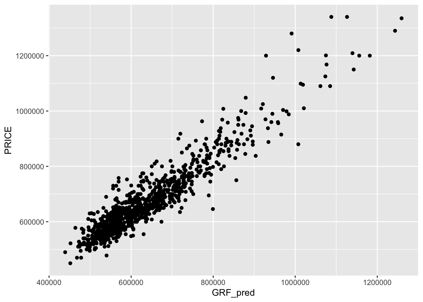
10 Conclusion
Lastly, we were task to compare the performance of the conventional OLS method versus the geographical weighted methods.
10.1 Differences between the two models
- OLS does not take into account the spatial autocorrelation whereas GRF does.
- Conventional OLS is generally good for exploratory data analysis but even so, more needs to be done to improve the model if it is meant to be used for prediction
We will compare the two models base on RMSE and on the visual plot.
rmse_lm[1] 87822.93test_data_lm <- cbind(test_data, lm_predicted_value)ggplot(data = test_data_lm,
aes(x = lm_predicted_value,
y = PRICE)) +
geom_point() +
geom_abline(col = "Red")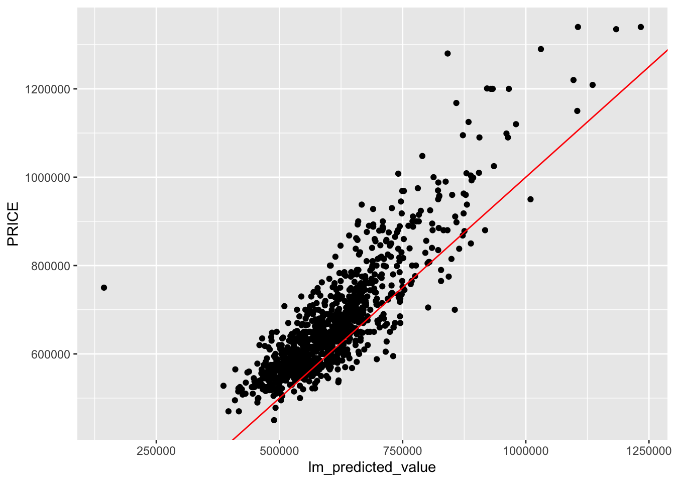
rmse_grf[1] 56235.78ggplot(data = test_data_p,
aes(x = GRF_pred,
y = PRICE)) +
geom_point()+
geom_abline(col = "Red")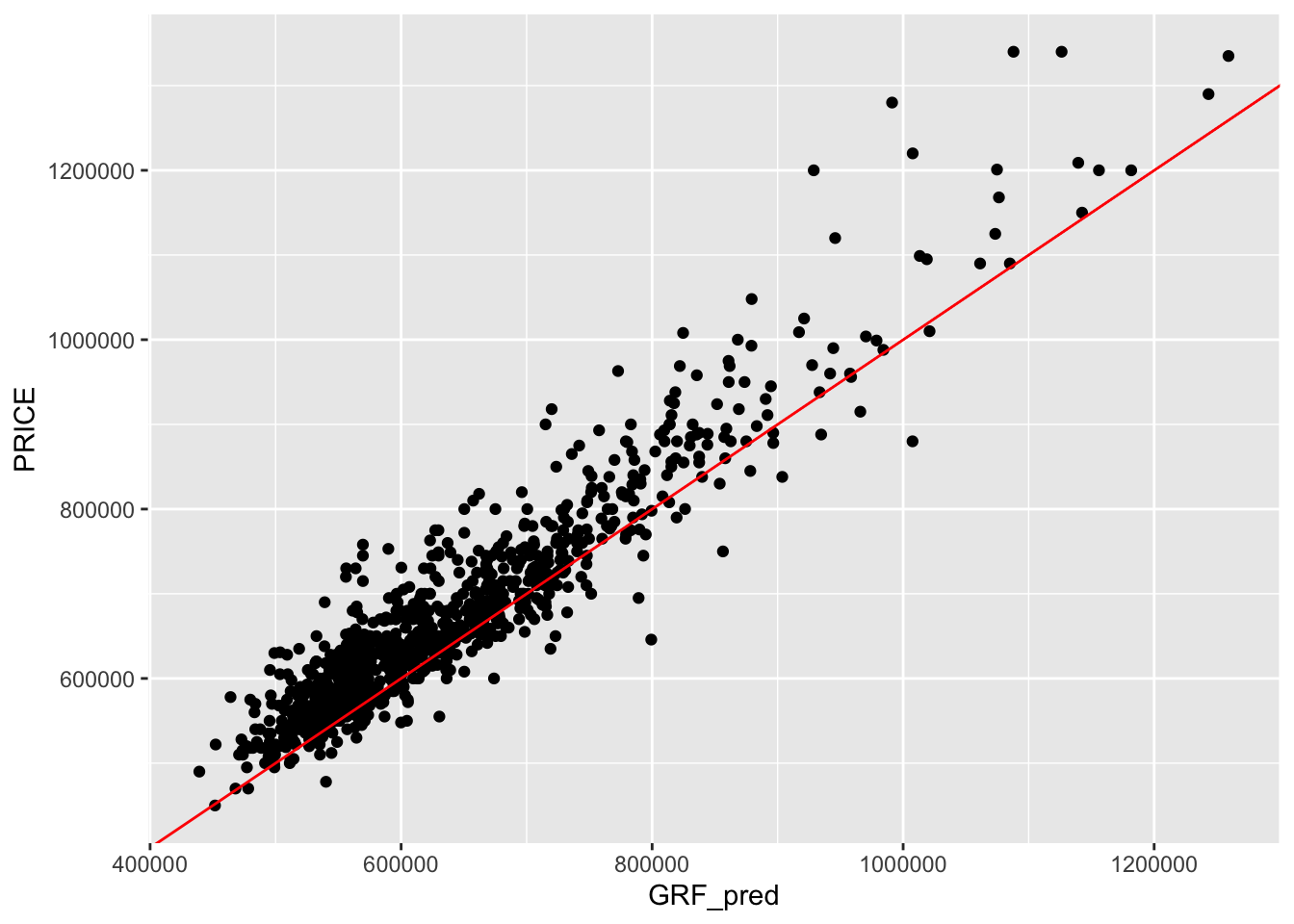
10.2 Predictive Power
By comparing the two models, we can see the RMSE for GRF, 56235.78, is lower than the RMSE for non-spatial regression, 87822.93. This suggest that the GRF Model is better at predicting the resale price.
Furthermore, we also notice that the points scattered in the GRF Model are clustered around the red line more than the non-spatial regression.
10.3 Limitations of Analysis
- One obvious limitation is the “sub-optimal” bandwidth generated for the GRF Model. This is due to the lack of computational power our devices have.
- Second is the number of trees that can be generated. Again for the same reason, I was only able to do ntree = 30. Having more trees may have better predictive power.
10.4 Possible Improvements to the model
- One way to improve the model could be the use of interactive variables.
Interactive variables helps to showcase the combined effects between two variables. For example, story_ordinal and NUM of primary school as an interactive variable. The intuition behind this is that primary schools generally contribute to higher noise-pollution and the higher the story level, the better as it can reduce the amount of noise that reaches the apartment. Such combined effects may improve the predictive power the model have.
Another example could be PROX_Parks and Story_Order. The closer one is to parks may signify better views. Higher story may allow residents to have better views and thus raise the price of the apartment. Again this is a useful variable to consider in our modelling.
- Removing outliers
While the regression helps us explain more than 90% of the variation in the Resale Price, there may be other reasons not captured affect the price. This could include sellers recent renovation of apartment, internal problems of the apartment and many others. Removing outliers may better fit the regression and reduce the prediction error.
However, outliers may have significant effect on the regression and may hold important information about the resale price. Hence, if the goal is to form a regression that is able to predict resale prices approximately, removing outliers in the training data may improve the model.
11 References
Much was referenced to Megan’s work on how to wrangle the data. Her work revolves around create hedonic model and it is a good read to understand how she goes through her assignment.
Prof Kam taught us several techniques on how to create the non-spatial regression as well as doing up the GRF modelling.